9. Structured Query Language (SQL)

Interactive SQL

This page uses MySQL. That means all the SQL code you see here is executed in your browser using WebAssembly. You can run the code snippets by clicking the "Run Code" button. If you want to run all the code snippets at once, click the "Run All" button.

Run All

Loading MySQL Console

“Any unique image that you desire probably already exists on the internet or in some database… The problem today is no longer how to create the right image, but how to find an already existing one”

Lev Manovich

In this Chapter

• Introduction
• Structured Query Language (SQL)
• Data Types and Constraints in MySQL
• SQL for Data Definition
• SQL for Data Manipulation
• SQL for Data Query
• Data Updation and Deletion
• Functions in SQL
• GROUP BY Clause in SQL
• Operations on Relations
• Using Two Relations in a Query

9.1 Introduction

We have learnt about Relational Database Management Systems (RDBMS) and its purpose in the previous chapter. There are many RDBMS such as MySQL, Microsoft SQL Server, PostgreSQL, Oracle, etc. that allow us to create a database consisting of relations. These RDBMS also allow us to store, retrieve and manipulate data on that database through queries. In this chapter, we will learn how to create, populate and query databases using MySQL.

9.2 Structured Query Language (SQL)

One has to write application programs to access data in case of a file system. However, for database management systems there are special kinds of languages called query language that can be used to access and manipulate data from the database. The Structured Query Language (SQL) is the most popular query language used by major relational database management systems such as MySQL, ORACLE, SQL Server, etc.

Activity 9.1

Find and list other types of databases other than RDBMS.

SQL is easy to learn as the statements comprise of descriptive English words and are not case sensitive. We can create and interact with a database using SQL easily. Benefit of using SQL is that we do not have to specify how to get the data from the database. Rather, we simply specify what is to be retrieved, and SQL does the rest. Although called a query language, SQL can do much more, besides querying. SQL provides statements for defining the structure of the data, manipulating data in the database, declaring constraints and retrieving data from the database in various ways, depending on our requirements.

In this chapter, we will use the StudentAttendance discussed in chapter 8 and create a database. We will also learn how to populate databases with data, manipulate data and retrieve data from a database through SQL queries.

9.2.1 Installing MySQL

MySQL is an open source RDBMS software which can be easily downloaded from the official website https://dev.mysql.com/downloads. After installing MySQL, start MySQL service. The appearance of mysql> prompt (Figure 9.1) means that MySQL is ready to accept SQL statements.

MySQL Shell 8.0 Command Line Client

Enter password: ****
Welcome to the MySQL monitor.  Commands end with ; or \g.
Your MySQL connection id is 11
Server version: 8.0.40 MySQL Community Server - GPL

Copyright (c) 2000, 2024, Oracle and/or its affiliates.

Oracle is a registered trademark of Oracle Corporation and/or its
affiliates. Other names may be trademarks of their respective
owners.

Type 'help;' or '\h' for help. Type '\c' to clear the current input statement.

mysql>

Figure 9.1: MySQL Shell

Following are some important points to be kept in mind while using SQL:

• SQL is case insensitive. For example, the column names ‘salary’ and ‘SALARY’ are the same for SQL.
• Always end SQL statements with a semicolon (;).
• To enter multiline SQL statements, we don’t write ; after the first line. We press the Enter key to continue on the next line. The prompt mysql> then changes to ->, indicating that statement is continued to the next line. After the last line, put ; and press enter.

9.3 Data Types and Constraints in MySQL

We know that a database consists of one or more relations and each relation (table) is made up of attributes (column). Each attribute has a data type. We can also specify constraints for each attribute of a relation.

9.3.1 Data type of Attribute

Data type of an attribute indicates the type of data value that an attribute can have. It also decides the operations that can be performed on the data of that attribute. For example, arithmetic operations can be performed on numeric data but not on character data. Commonly used data types in MySQL are numeric types, date and time types, and string types as shown in Table 9.1.

Table 9.1: Commonly used data types in MySQL

Data type	Description
CHAR(n)	Specifies character type data of length n where n could be any value from 0 to 1. CHAR is of fixed length, means, declaring CHAR(10) implies to reserve spaces for 10 characters. If data does not have 10 characters (e.g., ‘city’ has four characters), MySQL fills the remaining 6 characters with spaces padded on the right.
VARCHAR(n)	Specifies character type data of length where n could be any value from 0 to 65535. But unlike CHAR, VARCHAR(n) is a variable-length data type. That is, declaring VARCHAR(30) means a maximum of 30 characters can be stored but the actual allocated bytes will depend on the length of entered string. So ‘city’ in VARCHAR(30) will occupy space needed to store 4 characters only.
INT	INT specifies an integer value. Each INT value occupies 4 bytes of storage. The range of unsigned values allowed in a 4 byte integer type are 0 to 4,294,967,295. For values larger than that, we have to use BIGINT, which occupies 8 bytes.
FLOAT	Holds numbers with decimal points. Each FLOAT value occupies 4 bytes.
DATE	The DATE type is used for dates in ‘YYYY-MM-DD’ format. YYYY is the 4 digit year, MM is the 2 digit month and DD is the 2 digit date. The supported range is ‘1000-01-01’ to ‘9999-12-31’.

Activity 9.2

What are the other data types supported in MySQL? Are there other variants of integer and float data type?

9.3.2 Constraints

Constraints are the certain types of restrictions on the data values that an attribute can have. Table 9.2 lists some of the commonly used constraints in SQL. They are used to ensure correctness of data. However, it is not mandatory to define constraints for each attribute of a table.

Table 9.2: Commonly used SQL Constraints

Constraint	Description
NOT NULL	Ensures that a column cannot have NULL values where NULL means missing/unknown/not applicable value.
UNIQUE	Ensures that all the values in a column are distinct/unique
DEFAULT	A default value specified for the column if no value is provided
PRIMARY KEY	The column which can uniquely identify each row/record in a table.
FOREIGN KEY	The column which refers to value of an attribute defined as primary key in another table

Think and Reflect

Which two constraints when applied together will produce a Primary Key constraint?

9.4 SQL for Data Definition

In order to be able to store data we need to first define the relation schema. Defining a schema includes creating a relation and giving name to a relation, identifying the attributes in a relation, deciding upon the datatype for each attribute and also specify the constraints as per the requirements. Sometimes, we may require to make changes to the relation schema also. SQL allows us to write statements for defining, modifying and deleting relation schemas. These are part of Data Definition Language (DDL).

We have already learned that the data are stored in relations or tables in a database. Hence, we can say that a database is a collection of tables. The Create statement is used to create a database and its tables (relations). Before creating a database, we should be clear about the number of tables the database will have, the columns (attributes) in each table along with the data type of each column, and its constraint, if any.

9.4.1 CREATE Database

To create a database, we use the CREATE DATABASE statement as shown in the following

Syntax:

CREATE DATABASE databasename;

To create a database called StudentAttendance, we will type following command at mysql prompt.

CREATE DATABASE StudentAttendance;

CREATE DATABASE StudentAttendance;

Query OK, 1 row affected (0.02 sec)

Note

In LINUX environment, names for database and tables are case-sensitive whereas in WINDOWS, there is no such differentiation. However, as a good practice, it is suggested to write database/table name in the same letter cases that were used at the time of their creation.

Activity 9.3

Type the statement show database; Does it show the name of StudentAttendance database?

A DBMS can manage multiple databases on one computer. Therefore, we need to select the database that we want to use. To know the names of existing databases, we use the statement SHOW DATABASES. From the listed databases, we can select the database to be used. Once the database is selected, we can proceed with creating tables or querying data.

In order to use the StudentAttendance database, the following SQL statement is required.

USE StudentAttendance;

USE StudentAttendance;

Database changed

Initially, the created database is empty. It can be checked by using the show tables statement that lists names of all the tables within a database.

SHOW TABLES;

SHOW TABLES;

Empty set (0.06 sec)

9.4.2 CREATE Table

After creating a database StudentAttendance, we need to define relations in this database and specify attributes for each relation along with data type and constraint (if any) for each attribute. This is done using the CREATE TABLE statement.

Syntax:

CREATE TABLE tablename(
    attributename1 DATATYPE CONSTRAINT,
    attributename2 DATATYPE CONSTRAINT,
    :
    attributenameN DATATYPE CONSTRAINT
);

It is important to observe the following points with respect to the CREATE TABLE statement:

• The number of columns in a table defines the degree of that relation, which is denoted by N.
• Attribute name specifies the name of the column in the table.
• Datatype specifies the type of data that an attribute can hold.
• Constraint indicates the restrictions imposed on the values of an attribute. By default, each attribute can take NULL values except for the primary key.

Let us identify data types of the attributes of table STUDENT along with their constraints (if any). Assuming maximum students in a class to be 100 and values of roll number in a sequence from 1 to 100, we know that 3 digits are sufficient to store values for the attribute RollNumber. Hence, data type INT is appropriate for this attribute. Total number of characters in a student name (SName) can differ. Assuming maximum characters in a name as 20, we use VARCHAR(20) for the SName column. Data type for the attribute SDateofBirth is DATE and supposing the school uses guardian’s 12 digit Aadhaar number as GUID, we can declare GUID as CHAR (12) since Aadhaar number is of fixed length and we are not going to perform any mathematical operation on GUID.

Table 9.3, 9.4 and 9.5 shows the chosen data type and constraint for each attribute of the relations STUDENT, GUARDIAN and ATTENDANCE, respectively.

Table 9.3: Data types and constraints for the attributes of relation STUDENT

Attribute Name	Data expected to be stored	Data type	Constraint
RollNumber	Numeric value consisting of maximum 3 digits	INT	PRIMARY KEY
SName	Variant length string of maximum 20 characters	VARCHAR(20)	NOT NULL
SDateofBirth	Date value	DATE	NOT NULL
GUID	Numeric value consisting of 12 digits	CHAR (12)	FOREIGN KEY

Table 9.4: Data types and constraints for the attributes of relation GUARDIAN

Attribute Name	Data expected to be stored	Data type	Constraint
GUID	Numeric value consisting of 12 digit Aadhaar number	CHAR (12)	PRIMARY KEY
GName	Variant length string of maximum 20 characters	VARCHAR(20)	NOT NULL
GPhone	Numeric value consisting of 10 digits	CHAR(10)	NULL UNIQUE
GAddress	Variant length String of size 30 characters	VARCHAR(30)	NOT NULL

Table 9.5: Data types and constraints for the attributes of relation ATTENDANCE

Attribute Name	Data expected to be stored	Data type	Constraint
AttendanceDate	Date value	DATE	PRIMARY KEY*
RollNumber	Numeric value consisting of maximum 3 digits	INT	PRIMARY KEY* FOREIGN KEY
AttendanceStatus	’P’ for present and ‘A’ for absent	CHAR(1)	NOT NULL

*means part of composite primary key.

Once data types and constraints are identified, let us create tables without specifying constraints along with the attribute name for simplification. We will learn to incorporate constraints on attributes in Section 9.4.4.

Think and Reflect

Which datatype out of Char and Varchar will you prefer for storing contact number(mobile number)? Discuss.

Example 9.1

Create table STUDENT.

CREATE TABLE STUDENT(
    RollNumber INT,
    SName VARCHAR(20),
    SDateofBirth DATE,
    GUID CHAR (12),
    PRIMARY KEY (RollNumber)
);

CREATE TABLE STUDENT( RollNumber INT, SName VARCHAR(20), SDateofBirth DATE, GUID CHAR (12), PRIMARY KEY (RollNumber) );

Query OK, 0 rows affected (0.91 sec)

Note

“,” is used to separate two attributes and each statement terminates with a semi-colon (;). The arrow (->) is an interactive continuation prompt. If we enter an unfinished statement, the SQL shell will wait for us to enter the rest of the statement.

9.4.3 DESCRIBE Table

We can view the structure of an already created table using the DESCRIBE statement or DESC statement.

Syntax:

DESCRIBE tablename;

DESCRIBE STUDENT;

DESCRIBE STUDENT;

+--------------+-------------+------+-----+---------+-------+
| Field        | Type        | Null | Key | Default | Extra |
+--------------+-------------+------+-----+---------+-------+ 
| RollNumber   | int         | NO   | PRI | NULL    |       |
| SName        | varchar(20) | YES  |     | NULL    |       |
| SDateofBirth | date        | YES  |     | NULL    |       |
| GUID         | char(12)    | YES  |     | NULL    |       |
+--------------+-------------+------+-----+---------+-------+
4 rows in set (0.06 sec)

We can use the SHOW TABLES statement to see the tables in the StudentAttendance database. So far, we have only the STUDENT table.

SHOW TABLES;

SHOW TABLES;

+------------------------------+
| Tables_in_studentattendance  |
+------------------------------+
| student                      |
+------------------------------+
1 row in set (0.00 sec)

Activity 9.4

Create the other two relations GUARDIAN and ATTENDANCE as per data types given in Table 9.4 and 9.5 respectively, and view their structures. Do not add any constraint in these two tables.

9.4.4 ALTER Table

After creating a table, we may realise that we need to add/remove an attribute or to modify the datatype of an existing attribute or to add constraint in attribute. In all such cases, we need to change or alter the structure (schema) of the table by using the alter statement.

(A) Add primary key to a relation

Let us now alter the tables created in Activity 9.4. The following MySQL statement adds a primary key to the GUARDIAN relation:

Create GUARDIAN and ATTENDANCE tables

CREATE TABLE GUARDIAN (
    GUID CHAR(12),
    GName VARCHAR(20),
    GPhone CHAR(10),
    GAddress VARCHAR(30)
);
CREATE TABLE ATTENDANCE (
    AttendanceDate DATE,
    RollNumber INT,
    AttendanceStatus CHAR(1)
);

CREATE TABLE GUARDIAN ( GUID CHAR(12), GName VARCHAR(20), GPhone CHAR(10), GAddress VARCHAR(30) ); CREATE TABLE ATTENDANCE ( AttendanceDate DATE, RollNumber INT, AttendanceStatus CHAR(1) );

ALTER TABLE GUARDIAN ADD PRIMARY KEY (GUID);

ALTER TABLE GUARDIAN ADD PRIMARY KEY (GUID);

Query OK, 0 rows affected (1.14 sec)
Records: 0 Duplicates: 0 Warnings: 0

Now let us add the primary key to the ATTENDANCE relation. The primary key of this relation is a composite key made up of two attributes - AttendanceDate and RollNumber.

ALTER TABLE ATTENDANCE
ADD PRIMARY KEY(AttendanceDate, RollNumber);

ALTER TABLE ATTENDANCE ADD PRIMARY KEY(AttendanceDate, RollNumber);

Query OK, 0 rows affected (0.52 sec)
Records: 0 Duplicates: 0 Warnings: 0

Activity 9.5

Add foreign key in the ATTENDANCE table (use Figure 9.1) to identify referencing and referenced tables.

(B) Add foreign key to a relation

Once primary keys are added, the next step is to add foreign keys to the relation (if any). Following points need to be observed while adding foreign key to a relation:

• The referenced relation must be already created.
• The referenced attribute(s) must be part of the primary key of the referenced relation.
• Data types and size of referenced and referencing attributes must be the same.

Syntax:

ALTER TABLE table_name
ADD FOREIGN KEY(attribute_name)
REFERENCES referenced_table_name(attribute_name);

Let us now add foreign key to the table STUDENT. Table 9.3 shows that attribute GUID (the referencing attribute) is a foreign key and it refers to attribute GUID (the referenced attribute) of table GUARDIAN. Hence, STUDENT is the referencing table and GUARDIAN is the referenced table as shown in Figure 8.4 in the previous chapter.

ALTER TABLE STUDENT
ADD FOREIGN KEY(GUID)
REFERENCES GUARDIAN(GUID);

ALTER TABLE STUDENT ADD FOREIGN KEY(GUID) REFERENCES GUARDIAN(GUID);

Query OK, 0 rows affected (0.75 sec)
Records: 0 Duplicates: 0 Warnings: 0

Think and Reflect

Name foreign keys in table ATTENDANCE and STUDENT. Is there any foreign key in table GUARDIAN.

(C) Add constraint UNIQUE to an existing attribute

In GUARDIAN table, the attribute GPhone has a constraint UNIQUE which means no two values in that column should be the same.

Syntax:

ALTER TABLE table_name
ADD UNIQUE (attribute_name);

Let us now add the constraint UNIQUE with the attribute GPhone of the table GUARDIAN as shown at table 9.4.

ALTER TABLE GUARDIAN
ADD UNIQUE(GPhone);

ALTER TABLE GUARDIAN ADD UNIQUE(GPhone);

Query OK, 0 rows affected (0.44 sec)
Records: 0 Duplicates: 0 Warnings: 0

(D) Add an attribute to an existing table

Sometimes, we may need to add an additional attribute in a table. It can be done using the ADD attribute statement as shown in the following.

Syntax:

ALTER TABLE table_name
ADD attribute_name DATATYPE;

Suppose, the principal of the school has decided to award scholarship to some needy students for which income of the guardian must be known. But, the school has not maintained the income attribute with table GUARDIAN so far. Therefore, the database designer now needs to add a new attribute Income of data type INT in the table GUARDIAN.

ALTER TABLE GUARDIAN
ADD income INT;

ALTER TABLE GUARDIAN ADD income INT;

Query OK, 0 rows affected (0.47 sec)
Records: 0 Duplicates: 0 Warnings: 0

(E) Modify datatype of an attribute

We can change data types of the existing attributes of a table using the following ALTER statement.

Syntax:

ALTER TABLE table_name
MODIFY attribute DATATYPE;

Suppose we need to change the size of the attribute GAddress from VARCHAR(30) to VARCHAR(40) of the GUARDIAN table. The MySQL statement will be:

ALTER TABLE GUARDIAN
MODIFY GAddress VARCHAR(40);

ALTER TABLE GUARDIAN MODIFY GAddress VARCHAR(40);

Query OK, 0 rows affected (0.11 sec)
Records: 0 Duplicates: 0 Warnings: 0

(F) Modify constraint of an attribute

When we create a table, by default each attribute takes NULL value except for the attribute defined as primary key. We can change an attribute’s constraint from NULL to NOT NULL using an alter statement.

Syntax:

ALTER TABLE table_name
MODIFY attribute DATATYPE NOT NULL;

Note

We have to specify the data type of the attribute along with constraint NOT NULL while using MODIFY.

To associate NOT NULL constraint with attribute SName of table STUDENT (table 9.3), we write the following MySQL statement:

ALTER TABLE STUDENT
MODIFY SName VARCHAR(20) NOT NULL;

ALTER TABLE STUDENT MODIFY SName VARCHAR(20) NOT NULL;

Query OK, 0 rows affected (0.47 sec)
Records: 0 Duplicates: 0 Warnings: 0

Think and Reflect

What are the minimum and maximum income values that can be entered in the income attribute given the data type is INT?

(G) Add default value to an attribute

If we want to specify default value for an attribute, then use the following

Syntax:

ALTER TABLE table_name
MODIFY attribute DATATYPE DEFAULT default_value;

To set default value of SDateofBirth of STUDENT to 15th May 2000, write the following statement:

ALTER TABLE STUDENT
MODIFY SDateofBirth DATE DEFAULT '2000-05-15';

ALTER TABLE STUDENT MODIFY SDateofBirth DATE DEFAULT '2000-05-15';

Query OK, 0 rows affected (0.08 sec)
Records: 0 Duplicates: 0 Warnings: 0

Note

We have to specify the data type of the attribute along with DEFAULT while using MODIFY.

(H) Remove an attribute

Using ALTER, we can remove attributes from a table, as shown in the following

Syntax:

ALTER TABLE table_name
DROP attribute;

To remove the attribute income from table GUARDIAN (Table 9.4), write the following MySQL statement:

ALTER TABLE GUARDIAN DROP income;

ALTER TABLE GUARDIAN DROP income;

Query OK, 0 rows affected (0.42 sec)
Records: 0 Duplicates: 0 Warnings: 0

(I) Remove primary key from the table

Sometime there may be a requirement to remove primary key constraint from the table. In that case, ALTER TABLE command can be used in the following way:

Syntax:

ALTER TABLE table_name
DROP PRIMARY KEY;

To remove primary key of table GUARDIAN (Figure 9.4), write the following MySQL statement:

ALTER TABLE GUARDIAN DROP PRIMARY KEY;

ALTER TABLE GUARDIAN DROP PRIMARY KEY;

Query OK, 0 rows affected (0.72 sec)
Records: 0 Duplicates: 0 Warnings: 0

Note

We have dropped the primary key from the GUARDIAN table, but each table should have a primary key to maintain uniqueness. Hence, we have to use the ADD statement with the ALTER TABLE command to specify the primary key for the GUARDIAN table as shown in earlier examples.

9.4.5 DROP Statement

Sometimes a table in a database or the database itself needs to be removed. We can use a DROP statement to remove a database or a table permanently from the system. However, one should be very cautious while using this statement as it cannot be undone.

Syntax to drop a table:

DROP TABLE table_name;

Syntax to drop a database:

DROP DATABASE database_name;

Note

Using the DROP statement to remove a database will ultimately remove all the tables within it.

9.5 SQL for Data Manipulation

In the previous section, we created the database StudentAttendance having three relations STUDENT, GUARDIAN and ATTENDANCE. When we create a table, only its structure is created but the table has no data. To populate records in the table, INSERT statement is used. Also, table records can be deleted or updated using DELETE and UPDATE statements. These SQL statements are part of Data Manipulation Language (DML).

Data Manipulation using a database means either insertion of new data, removal of existing data or modification of existing data in the database

9.5.1 INSERTION of Records

INSERT INTO statement is used to insert new records in a table.

Its syntax is:

INSERT INTO tablename
VALUES(value 1, value 2,....);

Here, value 1 corresponds to attribute 1, value 2 corresponds to attribute 2 and so on. Note that we need not to specify attribute names in the insert statement if there are exactly the same numbers of values in the INSERT statement as the total number of attributes in the table.

Caution

While populating records in a table with foreign key, ensure that records in referenced tables are already populated.

Let us insert some records in the StudentAttendance database. We shall insert records in the GUARDIAN table first as it does not have any foreign key. A set of sample records for GUARDIAN table is shown in the given table (Table 9.6).

Table 9.6: Sample records for GUARDIAN table

GUID	GName	GPhone	GAddress
444444444444	Amit Ahuja	5711492685	G-35, Ashok Vihar, Delhi
111111111111	Baichung Bhutia	3612967082	Flat no. 5, Darjeeling Appt., Shimla
101010101010	Himanshu Shah	4726309212	26/77, West Patel Nagar, Ahmedabad
333333333333	Danny Dsouza		S -13, Ashok Village, Daman
466444444666	Sujata P.	3801923168	HNO-13, B- block, Preet Vihar, Madurai

The following insert statement adds the first record in the table:

INSERT INTO GUARDIAN
VALUES (
        444444444444,
        'Amit Ahuja',
        5711492685,
        'G-35,Ashok vihar, Delhi'
    );

INSERT INTO GUARDIAN VALUES ( 444444444444, 'Amit Ahuja', 5711492685, 'G-35,Ashok vihar, Delhi' );

Query OK, 1 row affected (0.01 sec)

Activity 9.6

Write SQL statements to insert the remaining 3 rows of table 9.6 in table GUARDIAN.

We can use the SQL statement SELECT * from table_name to view the inserted records. The SELECT statement will be explained in the next section.

SELECT * from  GUARDIAN;

SELECT * from GUARDIAN;

+--------------+------------+------------+-------------------------+
| GUID         | GName      | GPhone     | GAddress                |
+--------------+------------+------------+-------------------------+
| 444444444444 | Amit Ahuja | 5711492685 | G-35,Ashok vihar, Delhi |
+--------------+------------+------------+-------------------------+
1 row in set (0.01 sec)

If we want to insert values only for some of the attributes in a table (supposing other attributes having NULL or any other default value), then we shall specify the attribute names in which the values are to be inserted using the following syntax of INSERT INTO statement.

Syntax:

INSERT INTO tablename (column1, column2, ...)
VALUES (value1, value2,  ...);

To insert the fourth record of Table 9.6 where GPhone is not given, we need to insert values in the other three fields (GPhone was set to NULL by default at the time of table creation). In this case, we have to specify the names of attributes in which we want to insert values. The values must be given in the same order in which attributes are written in INSERT statement.

INSERT INTO GUARDIAN(GUID, GName, GAddress)
VALUES (
        333333333333,
        'Danny Dsouza',
        'S -13, Ashok Village, Daman'
    );

INSERT INTO GUARDIAN(GUID, GName, GAddress) VALUES ( 333333333333, 'Danny Dsouza', 'S -13, Ashok Village, Daman' );

Query OK, 1 row affected (0.03 sec)

Note

Text and date values must be enclosed in ' ' (single quotes).

SELECT * FROM GUARDIAN;

SELECT * FROM GUARDIAN;

+--------------+--------------+-----------+---------------------------+
| GUID         | GName        | Gphone    | GAddress                  |
+--------------+--------------+-----------+---------------------------+
| 333333333333 | Danny Dsouza | NULL      | S -13, Ashok Village,Daman|
| 444444444444 | Amit Ahuja   | 5711492685| G-35, Ashok vihar, Delhi  |
+--------------+--------------+-----------+---------------------------+
2 rows in set (0.00 sec)

Inserting remaining records in GUARDIAN table

INSERT INTO GUARDIAN
VALUES (
        111111111111,
        'Baichung Bhutia',
        3612967082,
        'Flat no. 5, Darjeeling Appt., Shimla'
    ),
    (
        101010101010,
        'Himanshu Shah',
        4726309212,
        '26/77, West Patel Nagar, Ahmedabad'
    ),
    (
        466444444666,
        'Sujata P.',
        3801923168,
        'HNO-13, B- block, Preet Vihar, Madurai'
    );
SELECT *
FROM GUARDIAN;

INSERT INTO GUARDIAN VALUES ( 111111111111, 'Baichung Bhutia', 3612967082, 'Flat no. 5, Darjeeling Appt., Shimla' ), ( 101010101010, 'Himanshu Shah', 4726309212, '26/77, West Patel Nagar, Ahmedabad' ), ( 466444444666, 'Sujata P.', 3801923168, 'HNO-13, B- block, Preet Vihar, Madurai' ); SELECT * FROM GUARDIAN;

Let us now insert the records given in Table 9.7 into the STUDENT table.

Table 9.7 STUDENT Table

RollNumber	SName	SDateofBirth	GUID
1	Atharv Ahuja	2003-05-15	444444444444
2	Daizy Bhutia	2002-02-28	111111111111
3	Taleem Shah	2002-02-28
4	John Dsouza	2003-08-18	333333333333
5	Ali Shah	2003-07-05	101010101010
6	Manika P.	2002-03-10	466444444666

Activity 9.7

Write SQL statements to insert the remaining 4 rows of table 9.7 in table STUDENT.

To insert the first record of Table 9.7, we write the following MySQL statement

INSERT INTO STUDENT
VALUES(
        1,
        'Atharv Ahuja',
        '2003-05-15',
        444444444444
    );

INSERT INTO STUDENT VALUES( 1, 'Atharv Ahuja', '2003-05-15', 444444444444 );

Query OK, 1 row affected (0.11 sec)

OR

INSERT INTO STUDENT (
        RollNumber,
        SName,
        SDateofBirth,
        GUID
    )
VALUES (
        1,
        'Atharv Ahuja',
        '2003-05-15',
        444444444444
    );

INSERT INTO STUDENT ( RollNumber, SName, SDateofBirth, GUID ) VALUES ( 1, 'Atharv Ahuja', '2003-05-15', 444444444444 );

Query OK, 1 row affected (0.02 sec)

Recall that Date is stored in ‘YYYY-MM-DD’ format.

SELECT * from STUDENT;

SELECT * from STUDENT;

+------------+--------------+--------------+--------------+
| RollNumber | SName        | SDateofBirth | GUID         |
+------------+--------------+--------------+--------------+
| 1          | Atharv Ahuja | 2003-05-15   | 444444444444 |
+------------+--------------+--------------+--------------+
1 row in set (0.00 sec)

Let us now insert the third record of Table 9.7 where GUID is NULL. Recall that GUID is foreign key of this table and thus can take NULL value. Hence, we can put NULL value for GUID and insert the record by using the following statement:

INSERT INTO STUDENT
VALUES(3, 'Taleem Shah','2002-02-28', NULL);

INSERT INTO STUDENT VALUES(3, 'Taleem Shah','2002-02-28', NULL);

Query OK, 1 row affected (0.05 sec)

SELECT * from STUDENT;

SELECT * from STUDENT;

+------------+--------------+--------------+--------------+
| RollNumber | SName        | SDateofBirth | GUID         |
+------------+--------------+--------------+--------------+
| 1          | Atharv Ahuja | 2003-05-15   | 444444444444 |
| 3          | Taleem Shah  | 2002-02-28   | NULL         |
+------------+--------------+--------------+--------------+
2 rows in set (0.00 sec)

We had to write NULL in the above insert statement because we are not mentioning the column names. Otherwise, we should mention the names of attributes along with the values if we need to insert data only for certain attributes, as shown in the following query:

INSERT INTO STUDENT (RollNumber, SName, SDateofBirth)
VALUES (3, 'Taleem Shah', '2002-02-28');

INSERT INTO STUDENT (RollNumber, SName, SDateofBirth) VALUES (3, 'Taleem Shah', '2002-02-28');

Query OK, 1 row affected (0.05 sec)

Inserting remaining records in STUDENT table

INSERT INTO STUDENT
VALUES (2, 'Daizy Bhutia', '2002-02-28', 111111111111),
    (4, 'John Dsouza', '2003-08-18', 333333333333),
    (5, 'Ali Shah', '2003-07-05', 101010101010),
    (6, 'Manika P.', '2002-03-10', 466444444666);
SELECT *
FROM STUDENT;

INSERT INTO STUDENT VALUES (2, 'Daizy Bhutia', '2002-02-28', 111111111111), (4, 'John Dsouza', '2003-08-18', 333333333333), (5, 'Ali Shah', '2003-07-05', 101010101010), (6, 'Manika P.', '2002-03-10', 466444444666); SELECT * FROM STUDENT;

Think and Reflect

• Which of the two insert statement should be used when the order of data to be inserted are not known?
• Can we insert two records with the same roll number?

9.6 SQL for Data Query

So far we have learnt how to create a database and how to store and manipulate data in them. We are interested in storing data in a database as it is easier to retrieve data in future from databases in whatever way we want. SQL provides efficient mechanisms to retrieve data stored in multiple tables in MySQL database (or any other RDBMS). The SQL statement SELECT is used to retrieve data from the tables in a database and is also called a query statement.

9.6.1 SELECT Statement

The SQL statement SELECT is used to retrieve data from the tables in a database and the output is also displayed in tabular form.

Syntax:

SELECT attribute1, attribute2, ...
FROM table_name
WHERE condition;

Here, attribute1, attribute2, … are the column names of the table table_name from which we want to retrieve data. The FROM clause is always written with SELECT clause as it specifies the name of the table from which data is to be retrieved. The WHERE clause is optional and is used to retrieve data that meet specified condition(s).

To select all the data available in a table, we use the following select statement:

SELECT * FROM table_name;

Example 9.2

The following query retrieves the name and date of birth of student with roll number 1:

SELECT SName,
    SDateofBirth
FROM STUDENT
WHERE RollNumber = 1;

SELECT SName, SDateofBirth FROM STUDENT WHERE RollNumber = 1;

+--------------+--------------+
| SName        | SDateofBirth |
+--------------+--------------+
| Atharv Ahuja | 2003-05-15   |
+--------------+--------------+
1 row in set (0.03 sec)

Think and Reflect

Think and list few examples from your daily life where storing the data in the database and querying the same can be helpful.

9.6.2 QUERYING using Database OFFICE

Organisations maintain databases to store data in the form of tables. Let us consider the database OFFICE of an organisation that has many related tables like EMPLOYEE, DEPARTMENT and so on. Every EMPLOYEE in the database is assigned to a DEPARTMENT and his/her Department number (DeptId) is stored as a foreign key in the table EMPLOYEE. Let us consider the relation ‘EMPLOYEE’ as shown in Table 9.8 and apply the SELECT statement to retrieve data:

Table 9.8: Records to be inserted into the EMPLOYEE table

EmpNo	Ename	Salary	Bonus	DeptId
101	Aaliya	10000	234	D02
102	Kritika	60000	123	D01
103	Shabbbir	45000	566	D01
104	Gurpreet	19000	565	D04
105	Joseph	34000	875	D03
106	Sanya	48000	695	D02
107	Vergese	15000		D01
108	Nachaobi	29000		D05
109	Daribha	42000		D04
110	Tanya	50000	467	D05

(A) Retrieve selected columns

The following query selects employee numbers of all the employees:

Create OFFICE database

CREATE DATABASE OFFICE;
USE OFFICE;
CREATE TABLE EMPLOYEE(
    EmpNo INT,
    Ename VARCHAR(20),
    Salary INT,
    Bonus INT,
    DeptId CHAR(3)
);
INSERT INTO EMPLOYEE (EmpNo, Ename, Salary, Bonus, DeptId)
VALUES (101, 'Aaliya', 10000, 234, 'D02'),
    (102, 'Kritika', 60000, 123, 'D01'),
    (103, 'Shabbbir', 45000, 566, 'D01'),
    (104, 'Gurpreet', 19000, 565, 'D04'),
    (105, 'Joseph', 34000, 875, 'D03'),
    (106, 'Sanya', 48000, 695, 'D02'),
    (107, 'Vergese', 15000, NULL, 'D01'),
    (108, 'Nachaobi', 29000, NULL, 'D05'),
    (109, 'Daribha', 42000, NULL, 'D04'),
    (110, 'Tanya', 50000, 467, 'D05');

CREATE DATABASE OFFICE; USE OFFICE; CREATE TABLE EMPLOYEE( EmpNo INT, Ename VARCHAR(20), Salary INT, Bonus INT, DeptId CHAR(3) ); INSERT INTO EMPLOYEE (EmpNo, Ename, Salary, Bonus, DeptId) VALUES (101, 'Aaliya', 10000, 234, 'D02'), (102, 'Kritika', 60000, 123, 'D01'), (103, 'Shabbbir', 45000, 566, 'D01'), (104, 'Gurpreet', 19000, 565, 'D04'), (105, 'Joseph', 34000, 875, 'D03'), (106, 'Sanya', 48000, 695, 'D02'), (107, 'Vergese', 15000, NULL, 'D01'), (108, 'Nachaobi', 29000, NULL, 'D05'), (109, 'Daribha', 42000, NULL, 'D04'), (110, 'Tanya', 50000, 467, 'D05');

SELECT EmpNo FROM EMPLOYEE;

SELECT EmpNo FROM EMPLOYEE;

+-------+
| EmpNo |
+-------+
| 101   |
| 102   |
| 103   |
| 104   |
| 105   |
| 106   |
| 107   |
| 108   |
| 109   |
| 110   |
+-------+
10 rows in set (0.41 sec)

The following query selects the employee number and employee name of all the employees, we write:

SELECT EmpNo, Ename FROM EMPLOYEE;

SELECT EmpNo, Ename FROM EMPLOYEE;

+-------+----------+
| EmpNo | Ename    |
+-------+----------+
| 101   | Aaliya   |
| 102   | Kritika  |
| 103   | Shabbir  |
| 104   | Gurpreet |
| 105   | Joseph   |
| 106   | Sanya    |
| 107   | Vergese  |
| 108   | Nachaobi |
| 109   | Daribha  |
| 110   | Tanya    | 
+-------+----------+
10 rows in set (0.00 sec)

(B) Renaming of columns

In case we want to rename any column while displaying the output, it can be done by using the alias AS. The following query selects Employee name as Name in the output for all the employees:

SELECT EName AS Name FROM EMPLOYEE;

SELECT EName AS Name FROM EMPLOYEE;

+----------+
| Name     |
+----------+
| Aaliya   |
| Kritika  |
| Shabbir  |
| Gurpreet |
| Joseph   |
| Sanya    |
| Vergese  |
| Nachaobi |
| Daribha  |
| Tanya    |
+----------+
10 rows in set (0.00 sec)

Example 9.3

Select names of all employees along with their annual income (calculated as Salary*12). While displaying the query result, rename the column EName as Name

SELECT EName AS Name,
    Salary * 12
FROM EMPLOYEE;

SELECT EName AS Name, Salary * 12 FROM EMPLOYEE;

+----------+-----------+
| Name     | Salary*12 |
+----------+-----------+
| Aaliya   | 120000    |
| Kritika  | 720000    |
| Shabbir  | 540000    |
| Gurpreet | 228000    |
| Joseph   | 408000    |
| Sanya    | 576000    |
| Vergese  | 180000    |
| Nachaobi | 348000    |
| Daribha  | 504000    |
| Tanya    | 600000    |
+----------+-----------+
10 rows in set (0.02 sec)

Observe that in the output, Salary*12 is displayed as the column name for the Annual Income column. In the output table, we can use alias to rename that column as Annual Income as shown below:

SELECT Ename AS Name,
    Salary * 12 AS 'Annual Income'
FROM EMPLOYEE;

SELECT Ename AS Name, Salary * 12 AS 'Annual Income' FROM EMPLOYEE;

+----------+---------------+
| Name     | Annual Income |
+----------+---------------+
| Aaliya   | 120000        |
| Kritika  | 720000        |
| Shabbir  | 540000        |
| Gurpreet | 228000        |
| Joseph   | 408000        |
| Sanya    | 576000        |
| Vergese  | 180000        |
| Nachaobi | 348000        |
| Daribha  | 504000        |
| Tanya    | 600000        |
+----------+---------------+
10 rows in set (0.00 sec)

Note

Annual Income will not be added as a new column in the database table. It is just for displaying the output of the query.

If an aliased column name has space as in the case of Annual Income, it should be enclosed in quotes as ‘Annual Income’.

(C) DISTINCT Clause

By default, SQL shows all the data retrieved through query as output. However, there can be duplicate values. The SELECT statement when combined with DISTINCT clause, returns records without repetition (distinct records). For example, while retrieving a department number from employee relation, there can be duplicate values as many employees are assigned to the same department. To select unique department number for all the employees, we use DISTINCT as shown below:

SELECT DISTINCT DeptId FROM EMPLOYEE;

SELECT DISTINCT DeptId FROM EMPLOYEE;

+--------+
| DeptId |
+--------+
| D02    |
| D01    |
| D04    |
| D03    |
| D05    |
+--------+
5 rows in set (0.03 sec)

(D) WHERE Clause

The WHERE clause is used to retrieve data that meet some specified conditions. In the OFFICE database, more than one employee can have the same salary. Following query gives distinct salaries of the employees working in the department number D01:

SELECT DISTINCT Salary
FROM EMPLOYEE
WHERE Deptid='D01';

SELECT DISTINCT Salary FROM EMPLOYEE WHERE Deptid='D01';

+--------+
| Salary |
+--------+
| 60000  |
| 45000  |
| 15000  |
+--------+
3 rows in set (0.02 sec)

As the column DeptId is of string type, its values are enclosed in quotes (‘D01’).

In the above example, = operator is used in the WHERE clause. Other relational operators (<, <=, >, >=, !=) can be used to specify such conditions. The logical operators AND, OR, and NOT are used to combine multiple conditions.

Example 9.4

Display all the details of those employees of D04 department who earn more than 5000.

SELECT *
FROM EMPLOYEE
WHERE Salary > 5000
    AND DeptId = 'D04';

SELECT * FROM EMPLOYEE WHERE Salary > 5000 AND DeptId = 'D04';

+-------+----------+--------+-------+--------+
| EmpNo | Ename    | Salary | Bonus | DeptId |
+-------+----------+--------+-------+--------+
| 104   | Gurpreet | 19000  | 565   | D04    |
| 109   | Daribha  | 42000  | NULL  | D04    |
+-------+----------+--------+-------+--------+
2 rows in set (0.00 sec)

Example 9.5

The following query selects records of all the employees except Aaliya.

SELECT *
FROM EMPLOYEE
WHERE NOT Ename = 'Aaliya';

SELECT * FROM EMPLOYEE WHERE NOT Ename = 'Aaliya';

+-------+----------+--------+-------+--------+
| EmpNo | Ename    | Salary | Bonus | DeptId |
+-------+----------+--------+-------+--------+
| 102   | Kritika  | 60000 | 123    | D01    |
| 103   | Shabbir  | 45000 | 566    | D01    |
| 104   | Gurpreet | 19000 | 565    | D04    |
| 105   | Joseph   | 34000 | 875    | D03    |
| 106   | Sanya    | 48000 | 695    | D02    |
| 107   | Vergese  | 15000 | NULL   | D01    |
| 108   | Nachaobi | 29000 | NULL   | D05    |
| 109   | Daribha  | 42000 | NULL   | D04    |
| 110   | Tanya    | 50000 | 467    | D05    |
+-------+----------+--------+-------+--------+
9 rows in set (0.00 sec)

Think and Reflect

What will happen if in the above query we write “Aaliya” as “AALIYA” or “aaliya” or “AaLIYA”? Will the query generate the same output or an error?

Example 9.6

The following query selects the name and department number of all those employees who are earning salary between 20000 and 50000 (both values inclusive).

SELECT Ename,
    DeptId
FROM EMPLOYEE
WHERE Salary >= 20000
    AND Salary <= 50000;

SELECT Ename, DeptId FROM EMPLOYEE WHERE Salary >= 20000 AND Salary <= 50000;

+----------+--------+
| Ename    | DeptId |
+----------+--------+
| Shabbir  | D01    |
| Joseph   | D03    |
| Sanya    | D02    |
| Nachaobi | D05    |
| Daribha  | D04    |
| Tanya    | D05    |
+----------+--------+
6 rows in set (0.00 sec)

SELECT * FROM EMPLOYEE
WHERE Salary > 5000 OR DeptId = 20;

SELECT * FROM EMPLOYEE WHERE Salary > 5000 OR DeptId = 20;

The query in example 9.6 defines a range that can also be checked using a comparison operator BETWEEN, as shown below:

SELECT Ename,
    DeptId
FROM EMPLOYEE
WHERE Salary BETWEEN 20000 AND 50000;

SELECT Ename, DeptId FROM EMPLOYEE WHERE Salary BETWEEN 20000 AND 50000;

+----------+--------+
| Ename    | DeptId |
+----------+--------+
| Shabbir  | D01    |
| Joseph   | D03    |
| Sanya    | D02    |
| Nachaobi | D05    |
| Daribha  | D04    |
| Tanya    | D05    |
+----------+--------+
6 rows in set (0.03 sec)

Note

The BETWEEN operator defines the range of values in which the column value must fall into, to make the condition true.

Activity 9.8

Compare the output produced by the query in Example 9.6 and the output of the following query and differentiate between the OR and AND operators.

Example 9.7

The following query selects details of all the employees who work in the departments having deptid D01, D02 or D04.

SELECT *
FROM EMPLOYEE
WHERE DeptId = 'D01'
    OR DeptId = 'D02'
    OR DeptId = 'D04';

SELECT * FROM EMPLOYEE WHERE DeptId = 'D01' OR DeptId = 'D02' OR DeptId = 'D04';

+-------+----------+--------+-------+--------+
| EmpNo | Ename    | Salary | Bonus | DeptId |
+-------+----------+--------+-------+--------+
| 101   | Aaliya   | 10000  | 234   | D02    |
| 102   | Kritika  | 60000  | 123   | D01    |
| 103   | Shabbir  | 45000  | 566   | D01    |
| 104   | Gurpreet | 19000  | 565   | D04    |
| 106   | Sanya    | 48000  | 695   | D02    |
| 107   | Vergese  | 15000  | NULL  | D01    |
| 109   | Daribha  | 42000  | NULL  | D04    | 
+-------+----------+--------+-------+--------+
7 rows in set (0.00 sec)

(E) Membership operator IN

The IN operator compares a value with a set of values and returns true if the value belongs to that set. The above query can be rewritten using IN operator as shown below:

SELECT *
FROM EMPLOYEE
WHERE DeptId IN ('D01', 'D02', 'D04');

SELECT * FROM EMPLOYEE WHERE DeptId IN ('D01', 'D02', 'D04');

+-------+----------+--------+-------+--------+
| EmpNo | Ename    | Salary | Bonus | DeptId |
+-------+----------+--------+-------+--------+
| 101   | Aaliya   | 10000  | 234   | D02    |
| 102   | Kritika  | 60000  | 123   | D01    |
| 103   | Shabbir  | 45000  | 566   | D01    |
| 104   | Gurpreet | 19000  | 565   | D04    |
| 106   | Sanya    | 48000  | 695   | D02    |
| 107   | Vergese  | 15000  | NULL  | D01    |
| 109   | Daribha  | 42000  | NULL  | D04    |
+-------+----------+--------+-------+--------+
7 rows in set (0.00 sec)

Example 9.8

The following query selects details of all the employees except those working in department number D01 or D02.

SELECT *
FROM EMPLOYEE
WHERE DeptId NOT IN('D01', 'D02');

SELECT * FROM EMPLOYEE WHERE DeptId NOT IN('D01', 'D02');

+-------+----------+--------+-------+--------+
| EmpNo | Ename    | Salary | Bonus | DeptId |
+-------+----------+--------+-------+--------+
| 104   | Gurpreet | 19000  | 565   | D04    |
| 105   | Joseph   | 34000  | 875   | D03    |
| 108   | Nachaobi | 29000  | NULL  | D05    |
| 109   | Daribha  | 42000  | NULL  | D04    |
| 110   | Tanya    | 50000  | 467   | D05    |
+-------+----------+--------+-------+--------+
5 rows in set (0.00 sec)

Note

Here we need to combine NOT with IN as we want to retrieve all records except with DeptId D01 and D02.

(F) ORDER BY Clause

ORDER BY clause is used to display data in an ordered form with respect to a specified column. By default, ORDER BY displays records in ascending order of the specified column’s values. To display the records in descending order, the DESC (means descending) keyword needs to be written with that column.

Example 9.9

The following query selects details of all the employees in ascending order of their salaries.

SELECT *
FROM EMPLOYEE
ORDER BY Salary;

SELECT * FROM EMPLOYEE ORDER BY Salary;

+-------+----------+--------+-------+--------+
| EmpNo | Ename    | Salary | Bonus | DeptId |
+-------+----------+--------+-------+--------+
| 101   | Aaliya   | 10000  | 234   | D02    |
| 107   | Vergese  | 15000  | NULL  | D01    |
| 104   | Gurpreet | 19000  | 565   | D04    |
| 108   | Nachaobi | 29000  | NULL  | D05    |
| 105   | Joseph   | 34000  | 875   | D03    |
| 109   | Daribha  | 42000  | NULL  | D04    |
| 103   | Shabbir  | 45000  | 566   | D01    |
| 106   | Sanya    | 48000  | 695   | D02    |
| 110   | Tanya    | 50000  | 467   | D05    |
| 102   | Kritika  | 60000  | 123   | D01    |
+-------+----------+--------+-------+--------+
10 rows in set (0.05 sec)

Example 9.10

Select details of all the employees in descending order of their salaries.

SELECT *
FROM EMPLOYEE
ORDER BY Salary DESC;

SELECT * FROM EMPLOYEE ORDER BY Salary DESC;

+-------+----------+--------+-------+--------+
| EmpNo | Ename    | Salary | Bonus | DeptId |
+-------+----------+--------+-------+--------+
| 102   | Kritika  | 60000  | 123   | D01    |
| 110   | Tanya    | 50000  | 467   | D05    |
| 106   | Sanya    | 48000  | 695   | D02    |
| 103   | Shabbir  | 45000  | 566   | D01    |
| 109   | Daribha  | 42000  | NULL  | D04    |
| 105   | Joseph   | 34000  | 875   | D03    |
| 108   | Nachaobi | 29000  | NULL  | D05    |
| 104   | Gurpreet | 19000  | 565   | D04    |
| 107   | Vergese  | 15000  | NULL  | D01    |
| 101   | Aaliya   | 10000  | 234   | D02    |
+-------+----------+--------+-------+--------+
10 rows in set (0.00 sec)

Activity 9.9

Execute the following 2 queries and find out what will happen if we specify two columns in the ORDER BY clause:

SELECT *
FROM EMPLOYEE
ORDER BY Salary,
    Bonus;

SELECT *
FROM EMPLOYEE
ORDER BY Salary,
    Bonus DESC;

(G) Handling NULL Values

SQL supports a special value called NULL to represent a missing or unknown value. For example, the Gphone column in the GUARDIAN table can have missing value for certain records. Hence, NULL is used to represent such unknown values. It is important to note that NULL is different from 0 (zero). Also, any arithmetic operation performed with NULL value gives NULL. For example: 5 + NULL = NULL because NULL is unknown hence the result is also unknown. In order to check for NULL value in a column, we use IS NULL operator.

Example 9.11

The following query selects details of all those employees who have not been given a bonus. This implies that the bonus column will be blank.

SELECT *
FROM EMPLOYEE
WHERE Bonus IS NULL;

SELECT * FROM EMPLOYEE WHERE Bonus IS NULL;

+-------+----------+--------+-------+--------+
| EmpNo | Ename    | Salary | Bonus | DeptId |
+-------+----------+--------+-------+--------+
| 107   | Vergese  | 15000  | NULL  | D01    |
| 108   | Nachaobi | 29000  | NULL  | D05    |
| 109   | Daribha  | 42000  | NULL  | D04    |
+-------+----------+--------+-------+--------+
3 rows in set (0.00 sec)

Example 9.12

The following query selects names of all employees who have been given a bonus (i.e., Bonus is not null) and works in the department D01.

SELECT EName
FROM EMPLOYEE
WHERE Bonus IS NOT NULL
    AND DeptID = 'D01';

SELECT EName FROM EMPLOYEE WHERE Bonus IS NOT NULL AND DeptID = 'D01';

+----------+
| EName    |
+----------+
| Kritika  |
| Shabbir  |
+----------+
2 rows in set (0.00 sec)

(H) Substring pattern matching

Many a times we come across situations where we do not want to query by matching exact text or value. Rather, we are interested to find matching of only a few characters or values in column values. For example, to find out names starting with “T” or to find out pin codes starting with ‘60’. This is called substring pattern matching. We cannot match such patterns using = operator as we are not looking for an exact match. SQL provides a LIKE operator that can be used with the WHERE clause to search for a specified pattern in a column.

The LIKE operator makes use of the following two wild card characters:

• % (per cent) - used to represent zero, one, or multiple characters

• _ (underscore) - used to represent exactly a single character

Think and Reflect

When we type first letter of a contact name in our contact list in our mobile phones all the names containing that character are displayed. Can you relate SQL statement with the process? List other real-life situations where you can visualise a SQL statement in operation.

Example 9.13

The following query selects details of all those employees whose name starts with ‘K’.

SELECT *
FROM EMPLOYEE
WHERE Ename like 'K%';

SELECT * FROM EMPLOYEE WHERE Ename like 'K%';

+-------+---------+--------+-------+--------+
| EmpNo | Ename   | Salary | Bonus | DeptId |
+-------+---------+--------+-------+--------+
| 102   | Kritika | 60000  | 123   | D01    |
+-------+---------+--------+-------+--------+
1 row in set (0.00 sec)

Example 9.14

The following query selects details of all those employees whose name ends with ‘a’, and gets a salary more than 45000.

SELECT *
FROM EMPLOYEE
WHERE Ename like '%a'
    AND Salary > 45000;

SELECT * FROM EMPLOYEE WHERE Ename like '%a' AND Salary > 45000;

+-------+---------+--------+-------+--------+
| EmpNo | Ename   | Salary | Bonus | DeptId |
+-------+---------+--------+-------+--------+
| 102   | Kritika | 60000  | 123   | D01    |
| 106   | Sanya   | 48000  | 695   | D02    |
| 110   | Tanya   | 50000  | 467   | D05    |
+-------+---------+--------+-------+--------+
3 rows in set (0.00 sec)

Example 9.15

The following query selects details of all those employees whose name consists of exactly 5 letters and starts with any letter but has ‘ANYA’ after that.

SELECT *
FROM EMPLOYEE
WHERE Ename like '_ANYA';

SELECT * FROM EMPLOYEE WHERE Ename like '_ANYA';

+-------+-------+--------+-------+--------+
| EmpNo | Ename | Salary | Bonus | DeptId |
+-------+-------+--------+-------+--------+
| 106   | Sanya | 48000  | 695   | D02    |
| 110   | Tanya | 50000  | 467   | D05    |
+-------+-------+--------+-------+--------+
2 rows in set (0.00 sec)

Example 9.16

The following query selects names of all employees containing ‘se’ as a substring in name.

SELECT Ename
FROM EMPLOYEE
WHERE Ename like '%se%';

SELECT Ename FROM EMPLOYEE WHERE Ename like '%se%';

+---------+
| Ename   |
+---------+
| Joseph  |
| Vergese |
+---------+
2 rows in set (0.00 sec)

Example 9.17

The following query selects names of all employees containing ‘a’ as the second character.

SELECT EName
FROM EMPLOYEE
WHERE Ename like '_a%';

SELECT EName FROM EMPLOYEE WHERE Ename like '_a%';

+----------+
| EName    |
+----------+
| Aaliya   |
| Sanya    |
| Nachaobi |
| Daribha  |
| Tanya    |
+----------+
5 rows in set (0.00 sec)

9.7 Data Updation and Deletion

Updation and deletion of data are also part of SQL Data Manipulation Language (DML). In this section, we are going to apply these two data manipulation methods on the StudentAttendance database given in section 9.4.

9.7.1 Data Updation

We may need to make changes in the value(s) of one or more columns of existing records in a table. For example, we may require some changes in address, phone number or spelling of name, etc. The UPDATE statement is used to make such modifications in existing data.

Syntax:

UPDATE table_name
SET attribute1 = value1,
    attribute2 = value2,
    ...
WHERE condition;

STUDENT Table 9.7 has NULL value in GUID for the student with roll number 3. Suppose students with roll numbers 3 and 5 are siblings. Then, in the STUDENT table, we need to fill the GUID value for the student with roll number 3 as 101010101010. In order to update or change GUID of a particular row (record), we need to specify that record using WHERE clause, as shown below:

Use StudentAttendance database

USE StudentAttendance;

USE StudentAttendance;

UPDATE STUDENT
SET GUID = 101010101010
WHERE RollNumber = 3;

UPDATE STUDENT SET GUID = 101010101010 WHERE RollNumber = 3;

Query OK, 1 row affected (0.06 sec) Rows matched: 1 
Changed: 1 Warnings: 0

We can then verify the updated data using the statement

SELECT * FROM STUDENT;

SELECT * FROM STUDENT;

Caution

If we miss the where clause in the UPDATE statement then the GUID of all the records will be changed to 101010101010.

We can also update values for more than one column using the UPDATE statement. Suppose, the guardian with GUID 466444444666 has requested to change Address to ‘WZ - 68, Azad Avenue, Bijnour, MP’ and Phone number to ‘4817362092’.

UPDATE GUARDIAN
SET GAddress = 'WZ - 68, Azad Avenue, Bijnour, MP',
    GPhone = 9010810547
WHERE GUID = 466444444666;

UPDATE GUARDIAN SET GAddress = 'WZ - 68, Azad Avenue, Bijnour, MP', GPhone = 9010810547 WHERE GUID = 466444444666;

Query OK, 1 row affected (0.06 sec)
Rows matched: 1 Changed: 1 Warnings: 0

SELECT * FROM GUARDIAN;

SELECT * FROM GUARDIAN;

+------------+---------------+------------+--------------------------------------+
|GUID        |GName          |Gphone      |GAddress                              |
+------------+---------------+------------+--------------------------------------+
|444444444444|Amit Ahuja     |5711492685  |G-35, Ashok vihar, Delhi              |
|111111111111|Baichung Bhutia|3612967082  |Flat no. 5, Darjeeling Appt., Shimla  |
|101010101010|Himanshu Shah  |4726309212  |26/77, West Patel Nagar, Ahmedabad    |
|333333333333|Danny Dsouza   |NULL        |S -13, Ashok Village, Daman           |
|466444444666|Sujata P.      |3801923168  |WZ - 68, Azad Avenue, Bijnour, MP     |
+------------+---------------+------------+--------------------------------------+
5 rows in set (0.00 sec)

9.7.2 Data Deletion

DELETE statement is used to delete/remove one or more records from a table.

Syntax:

DELETE FROM table_name
WHERE condition;

Suppose the student with roll number 2 has left the school. We can use the following MySQL statement to delete that record from the STUDENT table.

DELETE FROM STUDENT
WHERE RollNumber = 2;

DELETE FROM STUDENT WHERE RollNumber = 2;

Query OK, 1 row affected (0.06 sec)

SELECT * FROM STUDENT;

SELECT * FROM STUDENT;

+------------+--------------+--------------+--------------+
| RollNumber | SName        | SDateofBirth | GUID         |
+------------+--------------+--------------+--------------+
|          1 | Atharv Ahuja | 2003-05-15   | 444444444444 |
|          3 | Taleem Shah  | 2002-02-28   | 101010101010 |
|          4 | John Dsouza  | 2003-08-18   | 333333333333 |
|          5 | Ali Shah     | 2003-07-05   | 101010101010 |
|          6 | Manika P.    | 2002-03-10   | 466444444666 |
+------------+--------------+--------------+--------------+
5 rows in set (0.00 sec)

Caution

Like UPDATE statement, we need to be careful to include the WHERE clause while using a DELETE statement to delete records in a table. Otherwise, all the records in the table will get deleted.

9.8 Functions in SQL

In this section, we will understand how to use single row functions, multiple row functions, group records based on some criteria, and working on multiple tables using SQL.

Figure 9.2: Schema diagram of database CARSHOWROOM

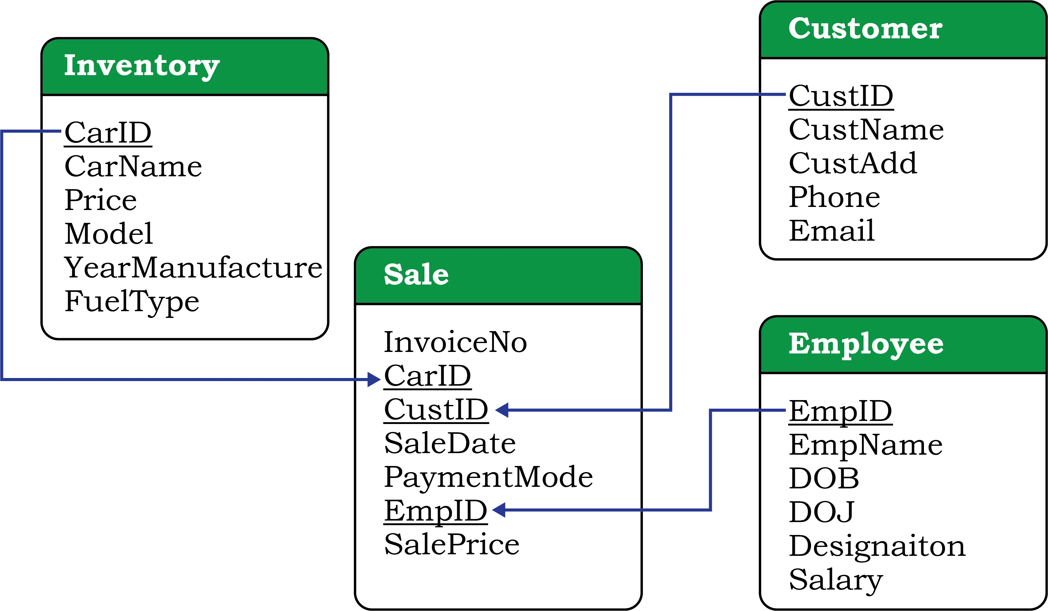
Let us create a database called CARSHOWROOM having the schema as shown in Figure 9.2 It has the following four relations:

1. INVENTORY: Stores name, price, model, year of manufacturing, and fuel type for each car in inventory of the showroom,

2. CUSTOMER: Stores customer id, name, address, phone number and email for each customer,

3. SALE: Stores the invoice number, car id, customer id, sale date, mode of payment, sales person’s employee id and selling price of the car sold,

4. EMPLOYEE: Stores employee id, name, date of birth, date of joining, designation and salary of each employee in the showroom.

Create CARSHOWROOM database

CREATE DATABASE CARSHOWROOM;
USE CARSHOWROOM;
CREATE TABLE INVENTORY (
    CarId VARCHAR(255) PRIMARY KEY,
    CarName VARCHAR(255),
    Price DECIMAL(10, 2),
    Model VARCHAR(255),
    YearManufacture INT,
    FuelType VARCHAR(255)
);
CREATE TABLE CUSTOMER (
    CustId VARCHAR(255) PRIMARY KEY,
    CustName VARCHAR(255),
    CustAdd VARCHAR(255),
    Phone VARCHAR(10),
    Email VARCHAR(255)
);
CREATE TABLE EMPLOYEE(
    EmpId VARCHAR(255) PRIMARY KEY,
    EmpName VARCHAR(255),
    DOB DATE,
    DOJ DATE,
    Designation VARCHAR(255),
    Salary INT
);
CREATE TABLE SALE (
    InvoiceNo VARCHAR(255) PRIMARY KEY,
    CarId VARCHAR(255),
    CustId VARCHAR(255),
    SaleDate DATE,
    PaymentMode VARCHAR(255),
    EmpId VARCHAR(255),
    SalePrice DECIMAL(10, 2),
    FOREIGN KEY (CarId) REFERENCES INVENTORY(CarId),
    FOREIGN KEY (CustId) REFERENCES CUSTOMER(CustId),
    FOREIGN KEY (EmpId) REFERENCES EMPLOYEE(EmpId)
);
INSERT INTO INVENTORY (
        CarId,
        CarName,
        Price,
        Model,
        YearManufacture,
        FuelType
    )
VALUES (
        'D001',
        'Dzire',
        582613.00,
        'LXI',
        2017,
        'Petrol'
    ),
    (
        'D002',
        'Dzire',
        673112.00,
        'VXI',
        2018,
        'Petrol'
    ),
    (
        'B001',
        'Baleno',
        567031.00,
        'Sigma1.2',
        2019,
        'Petrol'
    ),
    (
        'B002',
        'Baleno',
        647858.00,
        'Delta1.2',
        2018,
        'Petrol'
    ),
    (
        'E001',
        'EECO',
        355205.00,
        '5 STR STD',
        2017,
        'CNG'
    ),
    (
        'E002',
        'EECO',
        654914.00,
        'CARE',
        2018,
        'CNG'
    ),
    (
        'S001',
        'SWIFT',
        514000.00,
        'LXI',
        2017,
        'Petrol'
    ),
    (
        'S002',
        'SWIFT',
        614000.00,
        'VXI',
        2018,
        'Petrol'
    );
INSERT INTO CUSTOMER (
        CustId,
        CustName,
        CustAdd,
        Phone,
        Email
    )
VALUES (
        'C0001',
        'Amit Saha',
        'L-10, Pitampura',
        '4564587852',
        '[email protected]'
    ),
    (
        'C0002',
        'Rehnuma',
        'J-12, SAKET',
        '5527688761',
        '[email protected]'
    ),
    (
        'C0003',
        'Charvi Nayyar',
        '10/9, FF, Rohini',
        '6811635425',
        '[email protected]'
    ),
    (
        'C0004',
        'Gurpreet',
        'A-10/2, SF, Mayur Vihar',
        '3511056125',
        '[email protected]'
    );
INSERT INTO SALE (
        InvoiceNo,
        CarId,
        CustId,
        SaleDate,
        PaymentMode,
        EmpId,
        SalePrice
    )
VALUES (
        'I00001',
        'D001',
        'C0001',
        '2019-01-24',
        'Credit Card',
        'E004',
        613248.00
    ),
    (
        'I00002',
        'S001',
        'C0002',
        '2018-12-12',
        'Online',
        'E001',
        590321.00
    ),
    (
        'I00003',
        'S002',
        'C0004',
        '2019-01-25',
        'Cheque',
        'E010',
        604000.00
    ),
    (
        'I00004',
        'D002',
        'C0001',
        '2018-10-15',
        'Bank Finance',
        'E007',
        659982.00
    ),
    (
        'I00005',
        'E001',
        'C0003',
        '2018-12-20',
        'Credit Card',
        'E002',
        369310.00
    ),
    (
        'I00006',
        'S002',
        'C0002',
        '2019-01-30',
        'Bank Finance',
        'E007',
        620214.00
    );
INSERT INTO EMPLOYEE (
        EmpId,
        EmpName,
        DOB,
        DOJ,
        Designation,
        Salary
    )
VALUES (
        'E001',
        'Rushil',
        '1994-07-10',
        '2017-12-12',
        'Salesman',
        25550
    ),
    (
        'E002',
        'Sanjay',
        '1990-03-12',
        '2016-06-05',
        'Salesman',
        33100
    ),
    (
        'E003',
        'Zohar',
        '1975-08-30',
        '1999-01-08',
        'Peon',
        20000
    ),
    (
        'E004',
        'Arpit',
        '1989-06-06',
        '2010-12-02',
        'Salesman',
        39100
    ),
    (
        'E006',
        'Sanjucta',
        '1985-11-03',
        '2012-07-01',
        'Receptionist',
        27350
    ),
    (
        'E007',
        'Mayank',
        '1993-04-03',
        '2017-01-01',
        'Salesman',
        27352
    ),
    (
        'E010',
        'Rajkumar',
        '1987-02-26',
        '2013-10-23',
        'Salesman',
        31111
    );

CREATE DATABASE CARSHOWROOM; USE CARSHOWROOM; CREATE TABLE INVENTORY ( CarId VARCHAR(255) PRIMARY KEY, CarName VARCHAR(255), Price DECIMAL(10, 2), Model VARCHAR(255), YearManufacture INT, FuelType VARCHAR(255) ); CREATE TABLE CUSTOMER ( CustId VARCHAR(255) PRIMARY KEY, CustName VARCHAR(255), CustAdd VARCHAR(255), Phone VARCHAR(10), Email VARCHAR(255) ); CREATE TABLE EMPLOYEE( EmpId VARCHAR(255) PRIMARY KEY, EmpName VARCHAR(255), DOB DATE, DOJ DATE, Designation VARCHAR(255), Salary INT ); CREATE TABLE SALE ( InvoiceNo VARCHAR(255) PRIMARY KEY, CarId VARCHAR(255), CustId VARCHAR(255), SaleDate DATE, PaymentMode VARCHAR(255), EmpId VARCHAR(255), SalePrice DECIMAL(10, 2), FOREIGN KEY (CarId) REFERENCES INVENTORY(CarId), FOREIGN KEY (CustId) REFERENCES CUSTOMER(CustId), FOREIGN KEY (EmpId) REFERENCES EMPLOYEE(EmpId) ); INSERT INTO INVENTORY ( CarId, CarName, Price, Model, YearManufacture, FuelType ) VALUES ( 'D001', 'Dzire', 582613.00, 'LXI', 2017, 'Petrol' ), ( 'D002', 'Dzire', 673112.00, 'VXI', 2018, 'Petrol' ), ( 'B001', 'Baleno', 567031.00, 'Sigma1.2', 2019, 'Petrol' ), ( 'B002', 'Baleno', 647858.00, 'Delta1.2', 2018, 'Petrol' ), ( 'E001', 'EECO', 355205.00, '5 STR STD', 2017, 'CNG' ), ( 'E002', 'EECO', 654914.00, 'CARE', 2018, 'CNG' ), ( 'S001', 'SWIFT', 514000.00, 'LXI', 2017, 'Petrol' ), ( 'S002', 'SWIFT', 614000.00, 'VXI', 2018, 'Petrol' ); INSERT INTO CUSTOMER ( CustId, CustName, CustAdd, Phone, Email ) VALUES ( 'C0001', 'Amit Saha', 'L-10, Pitampura', '4564587852', '[email protected]' ), ( 'C0002', 'Rehnuma', 'J-12, SAKET', '5527688761', '[email protected]' ), ( 'C0003', 'Charvi Nayyar', '10/9, FF, Rohini', '6811635425', '[email protected]' ), ( 'C0004', 'Gurpreet', 'A-10/2, SF, Mayur Vihar', '3511056125', '[email protected]' ); INSERT INTO SALE ( InvoiceNo, CarId, CustId, SaleDate, PaymentMode, EmpId, SalePrice ) VALUES ( 'I00001', 'D001', 'C0001', '2019-01-24', 'Credit Card', 'E004', 613248.00 ), ( 'I00002', 'S001', 'C0002', '2018-12-12', 'Online', 'E001', 590321.00 ), ( 'I00003', 'S002', 'C0004', '2019-01-25', 'Cheque', 'E010', 604000.00 ), ( 'I00004', 'D002', 'C0001', '2018-10-15', 'Bank Finance', 'E007', 659982.00 ), ( 'I00005', 'E001', 'C0003', '2018-12-20', 'Credit Card', 'E002', 369310.00 ), ( 'I00006', 'S002', 'C0002', '2019-01-30', 'Bank Finance', 'E007', 620214.00 ); INSERT INTO EMPLOYEE ( EmpId, EmpName, DOB, DOJ, Designation, Salary ) VALUES ( 'E001', 'Rushil', '1994-07-10', '2017-12-12', 'Salesman', 25550 ), ( 'E002', 'Sanjay', '1990-03-12', '2016-06-05', 'Salesman', 33100 ), ( 'E003', 'Zohar', '1975-08-30', '1999-01-08', 'Peon', 20000 ), ( 'E004', 'Arpit', '1989-06-06', '2010-12-02', 'Salesman', 39100 ), ( 'E006', 'Sanjucta', '1985-11-03', '2012-07-01', 'Receptionist', 27350 ), ( 'E007', 'Mayank', '1993-04-03', '2017-01-01', 'Salesman', 27352 ), ( 'E010', 'Rajkumar', '1987-02-26', '2013-10-23', 'Salesman', 31111 );

The records of the four relations are shown in Tables 9.9, 9.10, 9.11, and 9.12, respectively.

Table 9.9: INVENTORY

SELECT * FROM INVENTORY;

SELECT * FROM INVENTORY;

+-------+---------+-----------+-----------+-----------------+----------+
| CarId | CarName | Price     | Model     | YearManufacture | FuelType |
+-------+---------+-----------+-----------+-----------------+----------+
| D001  | Dzire   | 582613.00 | LXI       |            2017 | Petrol   |
| D002  | Dzire   | 673112.00 | VXI       |            2018 | Petrol   |
| B001  | Baleno  | 567031.00 | Sigma1.2  |            2019 | Petrol   |
| B002  | Baleno  | 647858.00 | Delta1.2  |            2018 | Petrol   |
| E001  | EECO    | 355205.00 | 5 STR STD |            2017 | CNG      |
| E002  | EECO    | 654914.00 | CARE      |            2018 | CNG      |
| S001  | SWIFT   | 514000.00 | LXI       |            2017 | Petrol   |
| S002  | SWIFT   | 614000.00 | VXI       |            2018 | Petrol   |
+-------+---------+-----------+-----------+-----------------+----------+
8 rows in set (0.01 sec)

Table 9.10: CUSTOMER

SELECT * FROM CUSTOMER;

SELECT * FROM CUSTOMER;

+--------+---------------+-------------------------+------------+---------------------+
| CustId | CustName      | CustAdd                 | Phone      | Email               |
+--------+---------------+-------------------------+------------+---------------------+
| C0001  | Amit Saha     | L-10, Pitampura         | 4564587852 | [email protected] |
| C0002  | Rehnuma       | J-12, SAKET             | 5527688761 | [email protected] |
| C0003  | Charvi Nayyar | 10/9, FF, Rohini        | 6811635425 | [email protected] |
| C0004  | Gurpreet      | A-10/2, SF, Mayur Vihar | 3511056125 | [email protected] |
+--------+---------------+-------------------------+------------+---------------------+
4 rows in set (0.00 sec)

Table 9.11: SALE

SELECT * FROM SALE;

SELECT * FROM SALE;

+-----------+-------+--------+------------+--------------+-------+-----------+
| InvoiceNo | CarId | CustId | SaleDate   | PaymentMode  | EmpId | SalePrice |
+-----------+-------+--------+------------+--------------+-------+-----------+
| I00001    | D001  | C0001  | 2019-01-24 | Credit Card  | E004  | 613248.00 |
| I00002    | S001  | C0002  | 2018-12-12 | Online       | E001  | 590321.00 |
| I00003    | S002  | C0004  | 2019-01-25 | Cheque       | E010  | 604000.00 |
| I00004    | D002  | C0001  | 2018-10-15 | Bank Finance | E007  | 659982.00 |
| I00005    | E001  | C0003  | 2018-12-20 | Credit Card  | E002  | 369310.00 |
| I00006    | S002  | C0002  | 2019-01-30 | Bank Finance | E007  | 620214.00 |
+-----------+-------+--------+------------+--------------+-------+-----------+
6 rows in set (0.01 sec)

Table 9.12: EMPLOYEE

SELECT * FROM EMPLOYEE;

SELECT * FROM EMPLOYEE;

+-------+----------+------------+------------+--------------+--------+
| EmpId | EmpName  | DOB        | DOJ        | Designation  | Salary |
+-------+----------+------------+------------+--------------+--------+
| E001  | Rushil   | 1994-07-10 | 2017-12-12 | Salesman     |  25550 |
| E002  | Sanjay   | 1990-03-12 | 2016-06-05 | Salesman     |  33100 |
| E003  | Zohar    | 1975-08-30 | 1999-01-08 | Peon         |  20000 |
| E004  | Arpit    | 1989-06-06 | 2010-12-02 | Salesman     |  39100 |
| E006  | Sanjucta | 1985-11-03 | 2012-07-01 | Receptionist |  27350 |
| E007  | Mayank   | 1993-04-03 | 2017-01-01 | Salesman     |  27352 |
| E010  | Rajkumar | 1987-02-26 | 2013-10-23 | Salesman     |  31111 |
+-------+----------+------------+------------+--------------+--------+
7 rows in set (0.01 sec)

We know that a function is used to perform some particular task and it returns zero or more values as a result. Functions are useful while writing SQL queries also. Functions can be applied to work on single or multiple records (rows) of a table. Depending on their application in one or multiple rows, SQL functions are categorised as Single Row functions and Aggregate functions.

9.8.1 Single Row Functions

These are also known as Scalar functions. Single row functions are applied on a single value and return a single value. Figure 9.3 lists different single row functions under three categories — Numeric (Math), String, Date and Time.

Figure 9.3: Three categories of single-row functions in SQL

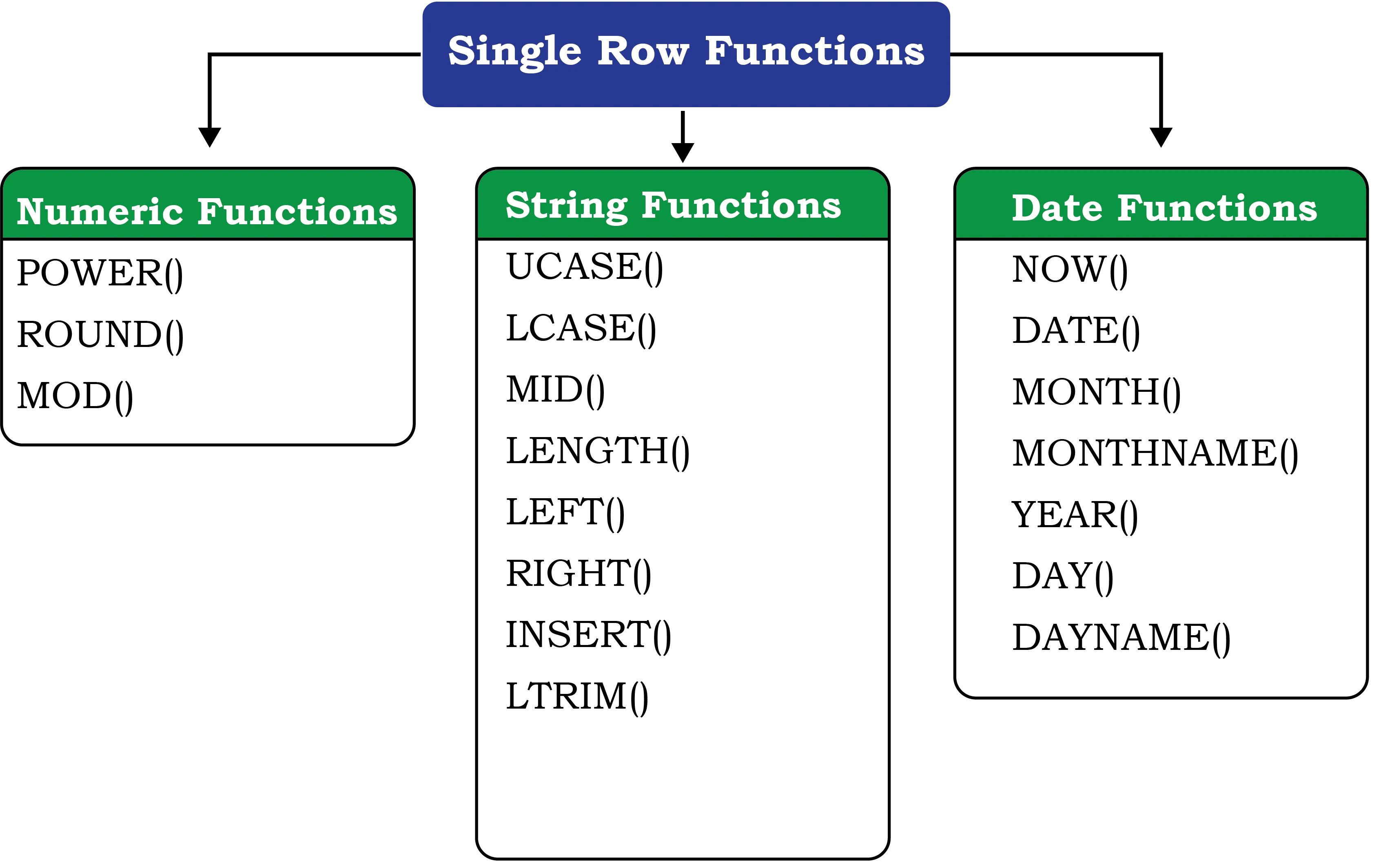
Math Functions accept numeric value as input and return a numeric value as a result. String Functions accept character value as input and return either character or numeric values as output. Date and Time functions accept date and time value as input and return numeric or string or Date and Time as output.

(A) Math Functions

Three commonly used numeric functions are POWER(), ROUND() and MOD(). Their usage along with syntax is given in Table 9.13.

Table 9.13: Math Functions

Function	Description	Example with output
POWER(X, Y)	Calculates X to the power Y.	SELECT POWER(2,3); SELECT POWER(2,3); 8
ROUND(N, D)	Rounds off number N to D number of decimal places. Note: If D=0, then it rounds off the number to the nearest integer.	SELECT ROUND(2912.564, 1); SELECT ROUND(2912.564, 1); 2912.6 SELECT ROUND(283.2); SELECT ROUND(283.2); 283
MOD(A, B)	Returns the remainder after dividing number A by number B.	SELECT MOD(21, 2); SELECT MOD(21, 2); 1

Activity 9.10

Using the table SALE of CARSHOWROOM database, write SQL queries for the following:

• a) Display the InvoiceNo and commission value rounded off to zero decimal places.
• b) Display the details of SALE where payment mode is credit card.

Example 9.18

In order to increase sales, suppose the car dealer decides to offer his customers to pay the total amount in 10 easy EMIs (equal monthly instalments). Assume that EMIs are required to be in multiples of 10000. For that, the dealer wants to list the CarID and Price along with the following data from the Inventory table:

• a) Calculate GST as 12 per cent of Price and display the result after rounding it off to one decimal place.

SELECT ROUND(12 / 100 * Price, 1) "GST"
FROM INVENTORY;

SELECT ROUND(12 / 100 * Price, 1) "GST" FROM INVENTORY;

+---------+
| GST     |
+---------+
| 69913.6 |
| 80773.4 |
| 68043.7 |
| 77743.0 |
| 42624.6 |
| 78589.7 |
| 61680.0 |
| 73680.0 |
+---------+
8 rows in set (0.01 sec)

• b) Add a new column FinalPrice to the table inventory which will have the value as sum of Price and 12 per cent of the GST.

ALTER TABLE INVENTORY
ADD(FinalPrice Numeric(10, 1));

ALTER TABLE INVENTORY ADD(FinalPrice Numeric(10, 1));

Query OK, 8 rows affected (0.03 sec)
Records: 8 Duplicates: 0 Warnings: 0

UPDATE INVENTORY
SET FinalPrice = Price + Round(Price * 12 / 100, 1);

UPDATE INVENTORY SET FinalPrice = Price + Round(Price * 12 / 100, 1);

Query OK, 8 rows affected (0.01 sec)
Rows matched: 8 Changed: 8 Warnings: 0

SELECT * FROM INVENTORY;

SELECT * FROM INVENTORY;

+-------+---------+-----------+-----------+-----------------+----------+------------+
| CarId | CarName | Price     | Model     | YearManufacture | FuelType | FinalPrice |
+-------+---------+-----------+-----------+-----------------+----------+------------+
| D001  | Dzire   | 582613.00 | LXI       |            2017 | Petrol   |   652526.6 |
| D002  | Dzire   | 673112.00 | VXI       |            2018 | Petrol   |   753885.4 |
| B001  | Baleno  | 567031.00 | Sigma1.2  |            2019 | Petrol   |   635074.7 |
| B002  | Baleno  | 647858.00 | Delta1.2  |            2018 | Petrol   |   725601.0 |
| E001  | EECO    | 355205.00 | 5 STR STD |            2017 | CNG      |   397829.6 |
| E002  | EECO    | 654914.00 | CARE      |            2018 | CNG      |   733503.7 |
| S001  | SWIFT   | 514000.00 | LXI       |            2017 | Petrol   |   575680.0 |
| S002  | SWIFT   | 614000.00 | VXI       |            2018 | Petrol   |   687680.0 |
+-------+---------+-----------+-----------+-----------------+----------+------------+
8 rows in set (0.02 sec)

• c) Calculate and display the amount to be paid each month (in multiples of 1000) which is to be calculated after dividing the FinalPrice of the car into 10 instalments.

• d) After dividing the amount into EMIs, find out the remaining amount to be paid immediately, by performing modular division.

Following SQL query can be used to solve the above mentioned (c) and (d) problem:

SELECT CarId,
    FinalPrice,
    ROUND(FinalPrice - MOD(FinalPrice, 1000) / 10, 0) "EMI",
    MOD(FinalPrice, 10000) "Remaining Amount"
FROM INVENTORY;

SELECT CarId, FinalPrice, ROUND(FinalPrice - MOD(FinalPrice, 1000) / 10, 0) "EMI", MOD(FinalPrice, 10000) "Remaining Amount" FROM INVENTORY;

+-------+------------+--------+------------------+
| CarId | FinalPrice | EMI    | Remaining Amount |
+-------+------------+--------+------------------+
| D001  |   652526.6 | 652474 |           2526.6 |
| D002  |   753885.4 | 753797 |           3885.4 |
| B001  |   635074.7 | 635067 |           5074.7 |
| B002  |   725601.0 | 725541 |           5601.0 |
| E001  |   397829.6 | 397747 |           7829.6 |
| E002  |   733503.7 | 733453 |           3503.7 |
| S001  |   575680.0 | 575612 |           5680.0 |
| S002  |   687680.0 | 687612 |           7680.0 |
+-------+------------+--------+------------------+
8 rows in set (0.04 sec)

Example 9.19

• a) Let us now add a new column Commission to the SALE table. The column Commission should have a total length of 7 in which 2 decimal places to be there.

ALTER TABLE SALE
ADD(Commission Numeric(7, 2));

ALTER TABLE SALE ADD(Commission Numeric(7, 2));

Query OK, 6 rows affected (0.34 sec)
Records: 6 Duplicates: 0 Warnings: 0

• b) Let us now calculate commission for sales agents as 12% of the SalePrice, Insert the values to the newly added column Commission and then display records of the table SALE where commission > 73000.

UPDATE SALE
SET Commission = 12 / 100 * SalePrice;

UPDATE SALE SET Commission = 12 / 100 * SalePrice;

Query OK, 6 rows affected (0.06 sec)
Rows matched: 6 Changed: 6 Warnings: 0

SELECT *
FROM SALE
WHERE Commission > 73000;

SELECT * FROM SALE WHERE Commission > 73000;

+-----------+-------+--------+------------+--------------+-------+-----------+------------+
| InvoiceNo | CarId | CustId | SaleDate   | PaymentMode  | EmpId | SalePrice | Commission |
+-----------+-------+--------+------------+--------------+-------+-----------+------------+
| I00001    | D001  | C0001  | 2019-01-24 | Credit Card  | E004  | 613248.00 |   73589.76 |
| I00004    | D002  | C0001  | 2018-10-15 | Bank Finance | E007  | 659982.00 |   79197.84 |
| I00006    | S002  | C0002  | 2019-01-30 | Bank Finance | E007  | 620214.00 |   74425.68 |
+-----------+-------+--------+------------+--------------+-------+-----------+------------+
3 rows in set (0.02 sec)

• c) Display InvoiceNo, SalePrice and Commission such that commission value is rounded off to 0.

SELECT InvoiceNo,
    SalePrice,
    Round(Commission, 0)
FROM SALE;

SELECT InvoiceNo, SalePrice, Round(Commission, 0) FROM SALE;

+-----------+-----------+----------------------+
| InvoiceNo | SalePrice | Round(Commission, 0) |
+-----------+-----------+----------------------+
| I00001    | 613248.00 |                73590 |
| I00002    | 590321.00 |                70839 |
| I00003    | 604000.00 |                72480 |
| I00004    | 659982.00 |                79198 |
| I00005    | 369310.00 |                44317 |
| I00006    | 620214.00 |                74426 |
+-----------+-----------+----------------------+
6 rows in set (0.01 sec)

Activity 9.11

Using the table INVENTORY from CARSHOWROOM database, write sql queries for the following:

• a) Convert the CarMake to uppercase if its value starts with the letter ‘B’.
• b) If the length of the car’s model is greater than 4 then fetch the substring starting from position 3 till the end from attribute Model.

(B) String Functions

String functions can perform various operations on alphanumeric data which are stored in a table. They can be used to change the case (uppercase to lowercase or vice-versa), extract a substring, calculate the length of a string and so on. String functions and their usage are shown in Table 9.14.

Table 9.14: String Functions

Function	Description	Example with output
UCASE(string) OR UPPER(string)	Converts string into uppercase.	SELECT UCASE("Informatics Practices"); SELECT UCASE("Informatics Practices"); INFORMATICS PRACTICES
LOWER(string) OR LCASE(string)	Converts string into lowercase.	SELECT LOWER("Informatics Practices"); SELECT LOWER("Informatics Practices"); informatics practices
MID(string, pos, n) OR SUBSTRING(string, pos, n) OR SUBSTR(string, pos, n)	Returns a substring of size n starting from the specified position (pos) of the string. If n is not specified, it returns the substring from the position pos till end of the string.	SELECT MID("Informatics", 3, 4); SELECT MID("Informatics", 3, 4); form SELECT MID('Informatics', 7); SELECT MID('Informatics', 7); atics
LENGTH(string)	Returns the number of characters in the specified string.	SELECT LENGTH("Informatics"); SELECT LENGTH("Informatics"); 11
LEFT(string, N)	Returns N number of characters from the left side of the string.	SELECT LEFT("Computer", 4); SELECT LEFT("Computer", 4); Comp
RIGHT(string, N)	Returns N number of characters from the right side of the string.	SELECT RIGHT("SCIENCE", 3); SELECT RIGHT("SCIENCE", 3); NCE
INSTR(string, substring)	Returns the position of the first occurrence of the substring in the given string. Returns 0, if the substring is not present in the string.	SELECT INSTR("Informatics", "ma"); SELECT INSTR("Informatics", "ma"); 6
LTRIM(string)	Returns the given string after removing leading white space characters.	SELECT LENGTH(" DELHI"), LENGTH(LTRIM(" DELHI")); SELECT LENGTH(" DELHI"), LENGTH(LTRIM(" DELHI")); 7, 5
RTRIM(string)	Returns the given string after removing trailing white space characters.	SELECT LENGTH("PEN "), LENGTH(RTRIM("PEN ")); SELECT LENGTH("PEN "), LENGTH(RTRIM("PEN ")); 5, 3
TRIM(string)	Returns the given string after removing both leading and trailing white space characters.	SELECT LENGTH(" MADAM "), LENGTH(TRIM(" MADAM ")); SELECT LENGTH(" MADAM "), LENGTH(TRIM(" MADAM ")); 9, 5

Activity 9.12

Using the table EMPLOYEE from CARSHOWROOM database, write SQL queries for the following:

• a) Display employee name and the last 2 characters of his EmpId.
• b) Display designation of employee and the position of character ‘e’ in designation, if present.

Example 9.20

Let us use Customer relation shown in Table 9.10 to understand the working of string functions.

• a) Display customer name in lower case and customer email in upper case from table CUSTOMER.

SELECT LOWER(CustName),
    UPPER(Email)
FROM CUSTOMER;

SELECT LOWER(CustName), UPPER(Email) FROM CUSTOMER;

+-----------------+---------------------+
| LOWER(CustName) | UPPER(Email)        |
+-----------------+---------------------+
| amit saha       | [email protected] |
| rehnuma         | [email protected] |
| charvi nayyar   | [email protected] |
| gurpreet        | [email protected] |
+-----------------+---------------------+
4 rows in set (0.01 sec)

• b) Display the length of the email and part of the email from the email id before the character ’@’. Note - Do not print ’@’.

SELECT LENGTH(Email),
    LEFT(Email, INSTR(Email, "@") -1)
FROM CUSTOMER;

SELECT LENGTH(Email), LEFT(Email, INSTR(Email, "@") -1) FROM CUSTOMER;

+---------------+-----------------------------------+
| LENGTH(Email) | LEFT(Email, INSTR(Email, "@") -1) |
+---------------+-----------------------------------+
|            19 | amitsaha2                         |
|            19 | rehnuma                           |
|            19 | charvi123                         |
|            19 | gur_singh                         |
+---------------+-----------------------------------+
4 rows in set (0.02 sec)

The function INSTR will return the position of ”@” in the email address. So, to print email id without ”@” we have to use position -1.

Activity 9.13

Using the table EMPLOYEE of CARSHOWROOM database, list the day of birth for all employees whose salary is more than 25000.

• c) Let us assume that four-digit area code is reflected in the mobile number starting from position number 3. For example, 1851 is the area code of mobile number 1. Now, write the SQL query to display the area code of the customer living in Rohini.

SELECT MID(Phone, 3, 4)
FROM CUSTOMER
WHERE CustAdd like '%Rohini%';

SELECT MID(Phone, 3, 4) FROM CUSTOMER WHERE CustAdd like '%Rohini%';

+------------------+
| MID(Phone, 3, 4) |
+------------------+
| 1163             |
+------------------+
1 row in set (0.02 sec)

Think and Reflect

Can we use arithmetic operators (+, -. *, or /) on date functions?

• d) Display emails after removing the domain name extension “.com” from emails of the customers.

SELECT TRIM(".com" FROM Email)
FROM CUSTOMER;

SELECT TRIM(".com" FROM Email) FROM CUSTOMER;

+-------------------------+
| TRIM(".com" FROM Email) |
+-------------------------+
| amitsaha2@gmail         |
| rehnuma@hotmail         |
| charvi123@yahoo         |
| gur_singh@yahoo         |
+-------------------------+
4 rows in set (0.00 sec)

• e) Display details of all the customers having yahoo emails only.

SELECT *
FROM CUSTOMER
WHERE Email LIKE "%yahoo%";

SELECT * FROM CUSTOMER WHERE Email LIKE "%yahoo%";

+--------+---------------+-------------------------+------------+---------------------+
| CustId | CustName      | CustAdd                 | Phone      | Email               |
+--------+---------------+-------------------------+------------+---------------------+
| C0003  | Charvi Nayyar | 10/9, FF, Rohini        | 6811635425 | [email protected] |
| C0004  | Gurpreet      | A-10/2, SF, Mayur Vihar | 3511056125 | [email protected] |
+--------+---------------+-------------------------+------------+---------------------+
2 rows in set (0.04 sec)

(C) Date and Time Functions

There are various functions that are used to perform operations on date and time data. Some of the operations include displaying the current date, extracting each element of a date (day, month and year), displaying day of the week and so on. Table 9.15 explains various date and time functions.

Table 9.15: Date Functions

Function	Description	Example with output
NOW()	It returns the current system date and time.	SELECT NOW(); SELECT NOW(); 2019-07-11 19:41:17
DATE()	It returns the date part from the given date/time expression.	SELECT DATE(NOW()); SELECT DATE(NOW()); 2019-07-11
MONTH(date)	It returns the month in numeric form from the date.	SELECT MONTH(NOW()); SELECT MONTH(NOW()); 7
MONTHNAME(date)	It returns the month name from the specified date.	SELECT MONTHNAME("2003-11-28"); SELECT MONTHNAME("2003-11-28"); November
YEAR(date)	It returns the year from the date.	SELECT YEAR("2003-10-03"); SELECT YEAR("2003-10-03"); 2003
DAY(date)	It returns the day part from the date.	SELECT DAY("2003-03-24"); SELECT DAY("2003-03-24"); 24
DAYNAME(date)	It returns the name of the day from the date.	SELECT DAYNAME("2019-07-11"); SELECT DAYNAME("2019-07-11"); Thursday

Activity 9.14

• a) Find sum of Sale Price of the cars purchased by the customer having ID C0001 from table SALE.
• b) Find the maximum and minimum commission from the SALE table.

Example 9.21

Let us use the EMPLOYEE table of CARSHOWROOM database to illustrate the working of some of the date and time functions.

• a) Select the day, month number and year of joining of all employees.

SELECT DAY(DOJ),
    MONTH(DOJ),
    YEAR(DOJ)
FROM EMPLOYEE;

SELECT DAY(DOJ), MONTH(DOJ), YEAR(DOJ) FROM EMPLOYEE;

+----------+------------+-----------+
| DAY(DOJ) | MONTH(DOJ) | YEAR(DOJ) |
+----------+------------+-----------+
|       12 |         12 |      2017 |
|        5 |          6 |      2016 |
|        8 |          1 |      1999 |
|        2 |         12 |      2010 |
|        1 |          7 |      2012 |
|        1 |          1 |      2017 |
|       23 |         10 |      2013 |
+----------+------------+-----------+
7 rows in set (0.02 sec)

• b) If the date of joining is not a Sunday, then display it in the following format “Wednesday, 26, November, 1979.”

SELECT DAYNAME(DOJ),
    DAY(DOJ),
    MONTHNAME(DOJ),
    YEAR(DOJ)
FROM EMPLOYEE
WHERE DAYNAME(DOJ) != 'Sunday';

SELECT DAYNAME(DOJ), DAY(DOJ), MONTHNAME(DOJ), YEAR(DOJ) FROM EMPLOYEE WHERE DAYNAME(DOJ) != 'Sunday';

+--------------+----------+----------------+-----------+
| DAYNAME(DOJ) | DAY(DOJ) | MONTHNAME(DOJ) | YEAR(DOJ) |
+--------------+----------+----------------+-----------+
| Tuesday      |       12 | December       |      2017 |
| Friday       |        8 | January        |      1999 |
| Thursday     |        2 | December       |      2010 |
| Wednesday    |       23 | October        |      2013 |
+--------------+----------+----------------+-----------+
4 rows in set (0.02 sec)

9.8.2 Aggregate Functions

Aggregate functions are also called Multiple Row functions. These functions work on a set of records as a whole and return a single value for each column of the records on which the function is applied. Table 9.16 shows the differences between single row functions and multiple row functions. Table 9.17 describes some of the aggregate functions along with their usage. Note that column must be of numeric type.

Table 9.16: Differences between Single and Multiple Row Functions

	Single Row Function	Multiple Row Function
1	It operates on a single row at a time.	It operates on groups of rows.
2	It returns one result per row.	It returns one result for a group of rows.
3	It can be used in Select, Where, and Order by clause.	It can be used in the select clause only.
4	Math, String and Date functions are examples of single row functions.	Max(), Min(), Avg(), Sum(), Count() and Count(*) are examples of multiple row functions.

Table 9.17: Aggregate Functions

Function	Description	Example with output
MAX(column)	Returns the largest value from the specified column.	SELECT MAX(Price) FROM INVENTORY; SELECT MAX(Price) FROM INVENTORY; 673112.00
MIN(column)	Returns the smallest value from the specified column.	SELECT MIN(Price) FROM INVENTORY; SELECT MIN(Price) FROM INVENTORY; 355205.00
AVG(column)	Returns the average of the values in the specified column.	SELECT AVG(Price) FROM INVENTORY; SELECT AVG(Price) FROM INVENTORY; 576091.625000
SUM(column)	Returns the sum of the values for the specified column.	SELECT SUM(Price) FROM INVENTORY; SELECT SUM(Price) FROM INVENTORY; 4608733.00
COUNT(*)	Returns the number of records in a table.	SELECT COUNT(*) FROM MANAGER; SELECT COUNT(*) FROM MANAGER; 4
COUNT(column)	Returns the number of values in the specified column ignoring the NULL values.	SELECT COUNT(MEMNAME) FROM MANAGER; SELECT COUNT(MEMNAME) FROM MANAGER; 3

Example 9.22

• a) Display the total number of records from table INVENTORY having a model as VXI.

SELECT COUNT(*)
FROM INVENTORY
WHERE Model = "VXI";

SELECT COUNT(*) FROM INVENTORY WHERE Model = "VXI";

+----------+
| COUNT(*) |
+----------+
|        2 |
+----------+
1 row in set (0.02 sec)

• b) Display the total number of different types of Models available from table INVENTORY.

SELECT COUNT(DISTINCT Model)
FROM INVENTORY;

SELECT COUNT(DISTINCT Model) FROM INVENTORY;

+-----------------------+
| COUNT(DISTINCT Model) |
+-----------------------+
|                     6 |
+-----------------------+
1 row in set (0.03 sec)

• c) Display the average price of all the cars with Model LXI from table INVENTORY.

SELECT AVG(Price)
FROM INVENTORY
WHERE Model = "LXI";

SELECT AVG(Price) FROM INVENTORY WHERE Model = "LXI";

+---------------+
| AVG(Price)    |
+---------------+
| 548306.500000 |
+---------------+
1 row in set (0.02 sec)

Activity 9.15

• a) List the total number of cars sold by each employee.
• b) List the maximum sale made by each employee.

9.9 GROUP BY Clause in SQL

At times we need to fetch a group of rows on the basis of common values in a column. This can be done using a group by clause. It groups the rows together that contains the same values in a specified column. We can use the aggregate functions (COUNT, MAX, MIN, AVG and SUM) to work on the grouped values. HAVING Clause in SQL is used to specify conditions on the rows with Group By clause.

Consider the SALE table from the CARSHOWROOM database:

SELECT * FROM SALE;

SELECT * FROM SALE;

+-----------+-------+--------+------------+--------------+-------+-----------+------------+
| InvoiceNo | CarId | CustId | SaleDate   | PaymentMode  | EmpId | SalePrice | Commission |
+-----------+-------+--------+------------+--------------+-------+-----------+------------+
| I00001    | D001  | C0001  | 2019-01-24 | Credit Card  | E004  | 613248.00 |   73589.76 |
| I00002    | S001  | C0002  | 2018-12-12 | Online       | E001  | 590321.00 |   70838.52 |
| I00003    | S002  | C0004  | 2019-01-25 | Cheque       | E010  | 604000.00 |   72480.00 |
| I00004    | D002  | C0001  | 2018-10-15 | Bank Finance | E007  | 659982.00 |   79197.84 |
| I00005    | E001  | C0003  | 2018-12-20 | Credit Card  | E002  | 369310.00 |   44317.20 |
| I00006    | S002  | C0002  | 2019-01-30 | Bank Finance | E007  | 620214.00 |   74425.68 |
+-----------+-------+--------+------------+--------------+-------+-----------+------------+
6 rows in set (0.03 sec)

CarID, CustID, SaleDate, PaymentMode, EmpID, SalePrice are the columns that can have rows with the same values in it. So, Group by clause can be used in these columns to find the number of records of a particular type (column), or to calculate the sum of the price of each car type.

Example 9.23

• a) Display the number of Cars purchased by each Customer from SALE table.

SELECT CustID,
    COUNT(*) "Number of Cars"
FROM SALE
GROUP BY CustID;

SELECT CustID, COUNT(*) "Number of Cars" FROM SALE GROUP BY CustID;

+--------+----------------+
| CustID | Number of Cars |
+--------+----------------+
| C0001  |              2 |
| C0002  |              2 |
| C0003  |              1 |
| C0004  |              1 |
+--------+----------------+
4 rows in set (0.03 sec)

• b) Display the Customer Id and number of cars purchased if the customer purchased more than 1 car from SALE table.

SELECT CustID,
    COUNT(*)
FROM SALE
GROUP BY CustID
HAVING Count(*) > 1;

SELECT CustID, COUNT(*) FROM SALE GROUP BY CustID HAVING Count(*) > 1;

+--------+----------+
| CustID | COUNT(*) |
+--------+----------+
| C0001  |        2 |
| C0002  |        2 |
+--------+----------+
2 rows in set (0.04 sec)

• c) Display the number of people in each category of payment mode from the table SALE.

SELECT PaymentMode,
    COUNT(PaymentMode)
FROM SALE
GROUP BY Paymentmode
ORDER BY Paymentmode;

SELECT PaymentMode, COUNT(PaymentMode) FROM SALE GROUP BY Paymentmode ORDER BY Paymentmode;

+--------------+--------------------+
| PaymentMode  | COUNT(PaymentMode) |
+--------------+--------------------+
| Bank Finance |                  2 |
| Cheque       |                  1 |
| Credit Card  |                  2 |
| Online       |                  1 |
+--------------+--------------------+
4 rows in set (0.04 sec)

• d) Display the PaymentMode and number of payments made using that mode more than once.

SELECT PaymentMode,
    Count(PaymentMode)
FROM SALE
GROUP BY Paymentmode
HAVING COUNT(*) > 1
ORDER BY Paymentmode;

SELECT PaymentMode, Count(PaymentMode) FROM SALE GROUP BY Paymentmode HAVING COUNT(*) > 1 ORDER BY Paymentmode;

+--------------+--------------------+
| PaymentMode  | Count(PaymentMode) |
+--------------+--------------------+
| Bank Finance |                  2 |
| Credit Card  |                  2 |
+--------------+--------------------+
2 rows in set (0.04 sec)

9.10 Operations on Relations

We can perform certain operations on relations like Union, Intersection and Set Difference to merge the tuples of two tables. These three operations are binary operations as they work upon two tables. Note here that these operations can only be applied if both the relations have the same number of attributes and corresponding attributes in both tables have the same domain.

9.10.1 UNION ($∪$)

This operation is used to combine the selected rows of two tables at a time. If some rows are same in both the tables, then result of the Union operation will show those rows only once. Figure 9.4 shows union of two sets.

Figure 9.4: Union of two sets

Let us consider two relations DANCE and MUSIC shown in Tables 9.18 and 9.19 respectively.

Table 9.18: DANCE

+------+--------+-------+
| SNo  | Name   | Class |
+------+--------+-------+
| 1    | Aastha | 7A    |
| 2    | Mahira | 6A    |
| 3    | Mohit  | 7B    |
| 4    | Sanjay | 7A    |
+------+--------+-------+

Table 9.19: MUSIC

+------+---------+-------+
| SNo  | Name    | Class |
+------+---------+-------+
| 1    | Mehak   | 8A    |
| 2    | Mahira  | 6A    |
| 3    | Lavanya | 7A    |
| 4    | Sanjay  | 7A    |
| 5    | Abhay   | 8A    |
+------+---------+-------+

If we need the list of students participating in either of events, then we have to apply UNION operation (represented by symbol $∪$) on relations DANCE and MUSIC. The output of UNION operation is shown in Table 9.20.

Table 9.20: DANCE U MUSIC

+------+---------+-------+
| SNo  | Name    | Class |
+------+---------+-------+
| 1    | Aastha  | 7A    |
| 2    | Mahira  | 6A    |
| 3    | Mohit   | 7B    |
| 4    | Sanjay  | 7A    |
| 1    | Mehak   | 8A    |
| 3    | Lavanya | 7A    |
| 5    | Abhay   | 8A    |
+------+---------+-------+

9.10.2 INTERSECT ($∩$)

Intersect operation is used to get the common tuples from two tables and is represented by symbol $∩$. Figure 9.5 shows intersection of two sets.

Figure 9.5: Intersection of two sets

Suppose, we have to display the list of students who are participating in both the events (DANCE and MUSIC), then intersection operation is to be applied on these two tables. The output of INTERSECT operation is shown in Table 9.21.

Table 9.21: DANCE ∩ MUSIC

+----+---------+-------+
| SNo| Name    | Class |
+----+---------+-------+
| 2  | Mahira  | 6A    |
| 4  | Sanjay  | 7A    |
+----+---------+-------+

9.10.3 MINUS ($-$)

This operation is used to get tuples/rows which are in the first table but not in the second table and the operation is represented by the symbol $-$ (minus). Figure 9.6 shows minus operation (also called set difference) between two sets.

Figure 9.6: Difference of two sets

Suppose we want the list of students who are only participating in MUSIC and not in DANCE event. Then, we will use the MINUS operation, whose output is given in Table 9.22.

Table 9.22: DANCE - MUSIC

+------+---------+-------+
| SNo  | Name    | Class |
+------+---------+-------+
| 1    | Mehak   | 8A    |
| 3    | Lavanya | 7A    |
| 5    | Abhay   | 8A    |
+------+---------+-------+

9.10.4 Cartesian Product ($×$)

Cartesian product operation combines tuples from two relations. It results in all pairs of rows from the two input relations, regardless of whether or not they have the same values on common attributes. It is denoted as '$×$'.

The degree of the resulting relation is calculated as the sum of the degrees of both the relations under consideration. The cardinality of the resulting relation is calculated as the product of the cardinality of relations on which cartesian product is applied. Let us use the relations DANCE and MUSIC to show the output of cartesian product. Note that both relations are of degree 1. The cardinality of relations DANCE and MUSIC is 4 and 5 respectively. Applying cartesian product on these two relations will result in a relation of degree 6 and cardinality 20, as shown in Table 9.23.

Table 9.23: DANCE × MUSIC

+---+--------+-------+------+---------+-------+
|SNo| Name   | Class | SNo  | Name    | Class |
+---+--------+-------+------+---------+-------+
| 1 | Aastha | 7A    | 1    | Mehak   | 8A    |
| 2 | Mahira | 6A    | 1    | Mehak   | 8A    |
| 3 | Mohit  | 7B    | 1    | Mehak   | 8A    |
| 4 | Sanjay | 7A    | 1    | Mehak   | 8A    |
| 1 | Aastha | 7A    | 2    | Mahira  | 6A    |
| 2 | Mahira | 6A    | 2    | Mahira  | 6A    |
| 3 | Mohit  | 7B    | 2    | Mahira  | 6A    |
| 4 | Sanjay | 7A    | 2    | Mahira  | 6A    |
| 1 | Aastha | 7A    | 3    | Lavanya | 7A    |
| 2 | Mahira | 6A    | 3    | Lavanya | 7A    |
| 3 | Mohit  | 7B    | 3    | Lavanya | 7A    |
| 4 | Sanjay | 7A    | 3    | Lavanya | 7A    |
| 1 | Aastha | 7A    | 4    | Sanjay  | 7A    |
| 2 | Mahira | 6A    | 4    | Sanjay  | 7A    |
| 3 | Mohit  | 7B    | 4    | Sanjay  | 7A    |
| 4 | Sanjay | 7A    | 4    | Sanjay  | 7A    |
| 1 | Aastha | 7A    | 5    | Abhay   | 8A    |
| 2 | Mahira | 6A    | 5    | Abhay   | 8A    |
| 3 | Mohit  | 7B    | 5    | Abhay   | 8A    |
| 4 | Sanjay | 7A    | 5    | Abhay   | 8A    |
+---+--------+-------+------+---------+-------+
20 rows in set (0.03 sec)

9.11 Using Two Relations in a Query

Till now we have written queries in SQL using a single relation only. In this section, we will learn to write queries using two relations.

9.11.1 Cartesian product on two tables

From the previous section, we learnt that application of operator cartesian product on two tables results in a table having all combinations of tuples from the underlying tables. When more than one table is to be used in a query, then we must specify the table names by separating commas in the FROM clause, as shown in Example 9.24. On execution of such a query, the DBMS (MySql) will first apply cartesian product on specified tables to have a single table. The following query of example 9.24 applies cartesian product on the two tables DANCE and MUSIC:

Example 9.24

Create CULTURE Database

CREATE DATABASE CULTURE;

USE CULTURE;

CREATE TABLE DANCE (
    SNo INT,
    Name VARCHAR(255),
    Class CHAR(2),
    PRIMARY KEY(SNo)
);

CREATE TABLE MUSIC(
    SNo INT,
    Name VARCHAR(255),
    Class CHAR(2),
    PRIMARY KEY(SNo)
);

INSERT INTO DANCE
VALUES (1, 'Aastha', '7A'),
    (2, 'Mahira', '6A'),
    (3, 'Mohit', '7B'),
    (4, 'Sanjay', '7A');

INSERT INTO MUSIC
VALUES (1, 'Mehak', '8A'),
    (2, 'Mahira', '6A'),
    (3, 'Lavanya', '7A'),
    (4, 'Sanjay', '7A'),
    (5, 'Abhay', '8A');

CREATE DATABASE CULTURE; USE CULTURE; CREATE TABLE DANCE ( SNo INT, Name VARCHAR(255), Class CHAR(2), PRIMARY KEY(SNo) ); CREATE TABLE MUSIC( SNo INT, Name VARCHAR(255), Class CHAR(2), PRIMARY KEY(SNo) ); INSERT INTO DANCE VALUES (1, 'Aastha', '7A'), (2, 'Mahira', '6A'), (3, 'Mohit', '7B'), (4, 'Sanjay', '7A'); INSERT INTO MUSIC VALUES (1, 'Mehak', '8A'), (2, 'Mahira', '6A'), (3, 'Lavanya', '7A'), (4, 'Sanjay', '7A'), (5, 'Abhay', '8A');

• a) Display all possible combinations of tuples of relations DANCE and MUSIC

SELECT *
FROM DANCE,
    MUSIC;

SELECT * FROM DANCE, MUSIC;

As we are using SELECT * in the query, the output will be the Table 9.23 having degree 6 and cardinality 20.

• b) From the all possible combinations of tuples of relations DANCE and MUSIC display only those rows such that the attribute name in both have the same value.

SELECT *
FROM DANCE D,
    MUSIC M
WHERE D.Name = M.Name;

SELECT * FROM DANCE D, MUSIC M WHERE D.Name = M.Name;

Table 9.24: Tuples with same name

+------+--------+-------+-----+--------+-------+
| Sno  | Name   | Class | Sno | Name   | class |
+------+--------+-------+-----+--------+-------+
| 2    | Mahira | 6A    | 2   | Mahira | 6A    |
| 4    | Sanjay | 7A    | 4   | Sanjay | 7A    |
+------+--------+-------+-----+--------+-------+
2 rows in set (0.00 sec)

Note that in this query we have used table aliases (D for DANCE and M for MUSIC), just like column aliases (see Section 9.6.2) to refer to tables by shortened names. It is important to note that table alias is valid only for current query and the original table name cannot be used in the query if its alias is given in FROM clause.

9.11.2 JOIN on two tables

JOIN operation combines tuples from two tables on specified conditions. This is unlike cartesian product which make all possible combinations of tuples. While using the JOIN clause of SQL, we specify conditions on the related attributes of two tables within the FROM clause. Usually, such an attribute is the primary key in one table and foreign key in another table. Let us create two tables UNIFORM (UCode, UName, UColor) and COST (UCode, Size, Price) in the SchoolUniform database. UCode is Primary Key in table UNIFORM. UCode and Size is the Composite Key in table COST. Therefore, Ucode is a common attribute between the two tables which can be used to fetch the common data from both tables. Hence, we need to define Ucode as foreign key in the Price table while creating this table.

Table 9.25: Uniform table

+-------+-------+--------+
| Ucode | Uname | Ucolor |
+-------+-------+--------+
| 1     | Shirt | White  |
| 2     | Pant  | Grey   |
| 3     | Tie   | Blue   |
+-------+-------+--------+

Table 9.26: Cost table

+-------+------+-------+
| Ucode | Size | Price |
+-------+------+-------+
| 1     | L    | 580   |
| 1     | M    | 500   |
| 2     | L    | 890   |
| 2     | M    | 810   |
+-------+------+-------+

Example 9.25

List the UCode, UName, UColor, Size and Price of related tuples of tables UNIFORM and COST.

Create UNIFORM Database

CREATE DATABASE UNIFORM;

USE UNIFORM;

CREATE TABLE UNIFORM (
    Ucode INT,
    Uname VARCHAR(255),
    Ucolor VARCHAR(255),
    PRIMARY KEY(Ucode)
);

CREATE TABLE COST(
    Ucode INT,
    Size CHAR(1),
    Price INT,
    PRIMARY KEY(Ucode, Size),
    FOREIGN KEY(Ucode) REFERENCES UNIFORM(Ucode)
);

INSERT INTO UNIFORM
VALUES (1, 'Shirt', 'White'),
    (2, 'Pant', 'Grey'),
    (3, 'Tie', 'Blue');

INSERT INTO COST
VALUES (1, 'L', 580),
    (1, 'M', 500),
    (2, 'L', 890),
    (2, 'M', 810);

CREATE DATABASE UNIFORM; USE UNIFORM; CREATE TABLE UNIFORM ( Ucode INT, Uname VARCHAR(255), Ucolor VARCHAR(255), PRIMARY KEY(Ucode) ); CREATE TABLE COST( Ucode INT, Size CHAR(1), Price INT, PRIMARY KEY(Ucode, Size), FOREIGN KEY(Ucode) REFERENCES UNIFORM(Ucode) ); INSERT INTO UNIFORM VALUES (1, 'Shirt', 'White'), (2, 'Pant', 'Grey'), (3, 'Tie', 'Blue'); INSERT INTO COST VALUES (1, 'L', 580), (1, 'M', 500), (2, 'L', 890), (2, 'M', 810);

The given query may be written in three different ways as given below.

• a) Using condition in where clause

SELECT *
FROM UNIFORM U,
    COST C
WHERE U.UCode = C.UCode;

SELECT * FROM UNIFORM U, COST C WHERE U.UCode = C.UCode;

Table 9.27: Output of the query

+-------+-------+--------+-------+------+-------+
| Ucode | Uname | Ucolor | Ucode | Size | Price |
+-------+-------+--------+-------+------+-------+
|     1 | Shirt | White  |     1 | L    |   580 |
|     1 | Shirt | White  |     1 | M    |   500 |
|     2 | Pant  | Grey   |     2 | L    |   890 |
|     2 | Pant  | Grey   |     2 | M    |   810 |
+-------+-------+--------+-------+------+-------+
4 rows in set (0.01 sec)

As the attribute Ucode is in both tables, we need to use table alias to remove ambiguity. Hence, we have used qualifier with attribute UCode in SELECT and FROM clauses to indicate its scope.

• b) Explicit use of JOIN clause

SELECT *
FROM UNIFORM U
    JOIN COST C ON U.Ucode = C.Ucode;

SELECT * FROM UNIFORM U JOIN COST C ON U.Ucode = C.Ucode;

The output of the query is same as shown in Table 9.26. In this query we have used JOIN clause explicitly along with condition in FROM clause. Hence no condition needs to be given in where clause.

• c) Explicit use of NATURAL JOIN clause

The output of queries (a) and (b) shown in Table 9.26 has a repetitive column Ucode having exactly the same values. This redundant column provides no additional information. There is an extension of JOIN operation called NATURAL JOIN which works similar to JOIN clause in SQL but removes the redundant attribute. This operator can be used to join the contents of two tables if there is one common attribute in both the tables. The above SQL query using NATURAL JOIN is shown below:

SELECT *
FROM UNIFORM
    NATURAL JOIN COST;

SELECT * FROM UNIFORM NATURAL JOIN COST;

+-------+-------+--------+------+-------+
| UCode | UName | UColor | Size | Price |
+-------+-------+--------+------+-------+
| 1     | Shirt | White  | L    | 580   |
| 1     | Shirt | White  | M    | 500   |
| 2     | Pant  | Grey   | L    | 890   |
| 2     | Pant  | Grey   | M    | 810   |
+-------+-------+--------+------+-------+
4 rows in set (0.17 sec)

It is clear from the output that the result of this query is same as that of queries written in (a) and (b) except that the attribute Ucode appears only once.

Following are some of the points to be considered while applying JOIN operations on two or more relations:

• If two tables are to be joined on equality condition on the common attribute, then one may use JOIN with ON clause or NATURAL JOIN in FROM clause. If three tables are to be joined on equality condition, then two JOIN or NATURAL JOIN are required.
• In general, $N-1$ joins are needed to combine $N$ tables on equality condition.
• With JOIN clause, we may use any relational operators to combine tuples of two tables.

---

Summary

• Database is a collection of related tables. MySQL is a ‘relational’ DBMS.

• DDL (Data Definition Language) includes SQL statements such as, Create table, Alter table and Drop table.

• DML (Data Manipulation Language) includes SQL statements such as, insert, select, update and delete.

• A table is a collection of rows and columns, where each row is a record and columns describe the feature of records.

• ALTER TABLE statement is used to make changes in the structure of a table like adding, removing or changing datatype of column(s).

• UPDATE statement is used to modify existing data in a table.

• WHERE clause in SQL query is used to enforce condition(s).

• DISTINCT clause is used to eliminate repetition and display the values only once.

• The BETWEEN operator defines the range of values inclusive of boundary values.

• The IN operator selects values that match any value in the given list of values.

• NULL values can be tested using IS NULL and IS NOT NULL.

• ORDER BY clause is used to display the result of a SQL query in ascending or descending order with respect to specified attribute values. By default, the order is ascending.

• LIKE operator is used for pattern matching. % and _ are two wild card characters. The per cent (%) symbol is used to represent zero or more characters. The underscore (_) symbol is used to represent a single character.

• A Function is used to perform a particular task and return a value as a result.

• Single Row functions work on a single row of the table and return a single value.

• Multiple Row functions work on a set of records as a whole and return a single value. Examples include COUNT, MAX, MIN, AVG and SUM.

• GROUP BY function is used to group rows of a table that contain the same values in a specified column.

• Join is an operation which is used to combine rows from two or more tables based on one or more common fields between them.

---

Exercise

Question 1

Answer the following questions:

• a) Define RDBMS. Name any two RDBMS software.

• b) What is the purpose of the following clauses in a select statement?

  • i) ORDER BY

  • ii) GROUP BY

• c) Site any two differences between Single Row Functions and Aggregate Functions.

• d) What do you understand by Cartesian Product?

• e) Differentiate between the following statements:

  • i) ALTER and UPDATE

  • ii) DELETE and DROP

• f) Write the name of the functions to perform the following operations:

  • i) To display the day like “Monday”, “Tuesday”, from the date when India got independence.

  • ii) To display the specified number of characters from a particular position of the given string.

  • iii) To display the name of the month in which you were born.

  • iv) To display your name in capital letters.

Question 2

Write the output produced by the following SQL statements:

• a)

  SELECT POW(2, 3);

• b)

  SELECT ROUND(342.9234, -1);

• c)

  SELECT LENGTH("Informatics Practices");

• d)

  SELECT YEAR("1979/11/26"),
      MONTH("1979/11/26"),
      DAY("1979/11/26"),
      MONTHNAME("1979/11/26");

• e)

  SELECT LEFT("INDIA", 3),
      RIGHT("Computer Science", 4),
      MID("Informatics", 3, 4),
      SUBSTR("Practices", 3);

Question 3

Consider the following MOVIE table and write the SQL queries based on it.

MovieID	MovieName	Category	ReleaseDate	ProductionCost	BusinessCost
001	Hindi_Movie	Musical	2018-04-23	124500	130000
002	Tamil_Movie	Action	2016-05-17	112000	118000
003	English_Movie	Horror	2017-08-06	245000	360000
004	Bengali_Movie	Adventure	2017-01-04	72000	100000
005	Telugu_Movie	Action	-	100000	-
006	Punjabi_Movie	Comedy	-	30500	-

• a) Display all the information from the Movie table.

• b) List business done by the movies showing only MovieID, MovieName and Total_Earning. Total_ Earning to be calculated as the sum of ProductionCost and BusinessCost.

• c) List the different categories of movies.

• d) Find the net profit of each movie showing its MovieID, MovieName and NetProfit. Net Profit is to be calculated as the difference between Business Cost and Production Cost.

• e) List MovieID, MovieName and Cost for all movies with ProductionCost greater than 10,000 and less than 1,00,000.

• f) List details of all movies which fall in the category of comedy or action.

• g) List details of all movies which have not been released yet.

Question 4

Suppose your school management has decided to conduct cricket matches between students of Class XI and Class XII. Students of each class are asked to join any one of the four teams - Team Titan, Team Rockers, Team Magnet and Team Hurricane. During summer vacations, various matches will be conducted between these teams. Help your sports teacher to do the following:

• a) Create a database “Sports”.

• b) Create a table “TEAM” with following considerations:

  • i) It should have a column TeamID for storing an integer value between 1 to 9, which refers to unique identification of a team.

  • ii) Each TeamID should have its associated name (TeamName), which should be a string of length not less than 10 characters.

• c) Using table level constraint, make TeamID as the primary key.

• d) Show the structure of the table TEAM using a SQL statement.

• e) As per the preferences of the students four teams were formed as given below. Insert these four rows in TEAM table:

  Row 1: (1, Team Titan)

  Row 2: (2, Team Rockers)

  Row 3: (3, Team Magnet)

  Row 3: (4, Team Hurricane)

• f) Show the contents of the table TEAM using a DML statement.

• g) Now create another table MATCH_DETAILS and insert data as shown below. Choose appropriate data types and constraints for each attribute.

Table: Match Details

MatchID	MatchDate	FirstTeamID	SecondTeamID	FirstTeamScore	SecondTeamScore
M1	2018-07-17	1	2	90	86
M2	2018-07-18	3	4	45	48
M3	2018-07-19	1	3	78	56
M4	2018-07-19	2	4	56	67
M5	2018-07-18	1	4	32	87
M6	2018-07-17	2	3	67	51

Question 5

Using the sports database containing two relations (TEAM, MATCH_DETAILS) and write the queries for the following:

• a) Display the MatchID of all those matches where both the teams have scored more than 70.

• b) Display the MatchID of all those matches where FirstTeam has scored less than 70 but SecondTeam has scored more than 70.

• c) Display the MatchID and date of matches played by Team 1 and won by it.

• d) Display the MatchID of matches played by Team 2 and not won by it.

• e) Change the name of the relation TEAM to T_DATA. Also change the attributes TeamID and TeamName to T_ID and T_NAME respectively.

Question 6

A shop called Wonderful Garments who sells school uniforms maintains a database SCHOOLUNIFORM as shown below. It consisted of two relations - UNIFORM and COST. They made UniformCode as the primary key for UNIFORM relations. Further, they used UniformCode and Size to be composite keys for COSTrelation. By analysing the database schema and database state, specify SQL queries to rectify the following anomalies.

• a) M/S Wonderful Garments also keeps handkerchiefs of red colour, medium size of Rs. 100 each.

• b)

  INSERT INTO COST (UCode, Size, Price)
  VALUES (7, 'M', 100);

  When the above query is used to insert data, the values for the handkerchief without entering its details in the UNIFORM relation is entered. Make a provision so that the data can be entered in the COST table only if it is already there in the UNIFORM table.

• c) Further, they should be able to assign a new UCode to an item only if it has a valid UName. Write a query to add appropriate constraints to the SCHOOLUNIFORM database.

• d) Add the constraint so that the price of an item is always greater than zero.

Question 7

Consider the following table named “Product”, showing details of products being sold in a grocery shop.

PCode	PName	UPrice	Manufacturer
P01	Washing Powder	120	Surf
P02	Toothpaste	54	Colgate
P03	Soap	25	Lux
P04	Toothpaste	65	Pepsodent
P05	Soap	38	Dove
P06	Shampoo	245	Dove

Write SQL queries for the following:

• a) Create the table Product with appropriate data types and constraints.

• b) Identify the primary key in Product.

• c) List the Product Code, Product name and price in descending order of their product name. If PName is the same, then display the data in ascending order of price.

• d) Add a new column Discount to the table Product.

• e) Calculate the value of the discount in the table Product as 10 per cent of the UPrice for all those products where the UPrice is more than 100, otherwise the discount will be 0.

• f) Increase the price by 12 per cent for all the products manufactured by Dove.

• g) Display the total number of products manufactured by each manufacturer.

Write the output(s) produced by executing the following queries on the basis of the information given above in the table Product:

• h)

  SELECT PName,
      avg(UPrice)
  FROM Product
  GROUP BY Pname;

• i)

  SELECT DISTINCT Manufacturer
  FROM Product;

• j)

  SELECT COUNT (DISTINCT PName)
  FROM Product;

• k)

  SELECT PName,
      MAX(UPrice),
      MIN(UPrice)
  FROM Product
  GROUP BY PName;

Question 8

Using the CARSHOWROOM database given in the chapter, write the SQL queries for the following:

• a) Add a new column Discount in the INVENTORY table.

• b) Set appropriate discount values for all cars keeping in mind the following:

  • (i) No discount is available on the LXI model.

  • (ii) VXI model gives a 10 per cent discount.

  • (iii) A 12 per cent discount is given on cars other than LXI model and VXI model.

• c) Display the name of the costliest car with fuel type “Petrol”.

• d) Calculate the average discount and total discount available on Baleno cars.

• e) List the total number of cars having no discount.

---